

© 2026 Wei Li · Homepedia. All rights reserved. The text, data and charts in this report are protected by copyright and may not be copied, republished, excerpted or used commercially without written permission.
Abstract
Boston is a housing market that looks as if it should not rise, yet keeps rising. Between 2019 and 2024, total employment in the Boston metro fell 0.5%, and in August 2026 it was still 2.0% below its late-2019 level. Finance, information and manufacturing each have more than 5% fewer jobs than before the pandemic; the metro loses 16,000 to 39,000 residents a year to the rest of the country; and the life-sciences industry that defines the city now has 21.2% lab vacancy and posted its first biopharma job decline in more than two decades. Over the same period, Boston’s typical home value rose 47.4% and set a new record in August 2026.
This report asks why a metro with almost no demand growth keeps setting price records, and where the limits of that resilience lie. Our central thesis—the one Wei Li stated on the SeaHomepedia Housing Map—is: health care, education and advanced research give Boston’s economy strong resilience, and near-zero new supply converts that resilience into stable home prices; but prices are now high enough to squeeze out new buyers, so rentals in the urban core are better supported than ordinary owner-occupied homes. That is a judgment about the next two years. This report also gives a ten-year judgment, and it points the other way: what holds up Boston’s prices is a pool of roughly 320,000 jobs paying $150,000 or more, 89% of them in management, finance, computing, engineering, science and law, occupations whose work is judgment; over the next decade AI is likely to take most of those jobs away, and supply that is scarce today will then amplify the contraction in demand into a fall in prices. The two-year path does not describe the ten-year path, and the two judgments must be read separately.
We test both judgments with 24 charts built from public data. Supply: in 2020–2025 the Boston metro permitted only 2.0–3.4 homes per 1,000 residents a year, a quarter to a third of Dallas’s rate; Saiz (2010) estimates Boston’s housing supply elasticity at just 0.86, the 15th lowest of 95 large metros. A 73-metro regression shows that in a low-elasticity market like Boston, each percentage point of job growth corresponds to about 2.3 points of price growth—any change in demand is amplified into prices. Demand: a typical home now requires about $195,000 of household income, 1.66 times the metro median; households leaving for other states earn 30% more on average ($131,000) than those arriving from other states ($101,000), so the pool of affluent marginal buyers is not growing. Price structure: suburbs and gateway cities lead while the core lags—since 2019, Lowell and Plymouth are up 59–65%, Boston proper only 15.9% and Brookline only 7.0%; yet in those same core towns rents rose 25–38%, about twice as fast as home values.
Our base case is “resilient divergence”: over the next 12–24 months, supply constraints keep supporting overall prices while affordability keeps sales volume low; ordinary owner-occupied homes in the suburbs and gateway cities hold up, owner-occupied product in the core (especially condos) keeps underperforming, and core rental demand stays firm. The largest downside risk is a further contraction in federal research funding and life-sciences financing.
The ten-year picture is different. The 320,000 jobs in occupations paying $150,000 or more account for 27% of Boston’s payroll (12% nationally), and 284,000 of them are in judgment-based occupational groups; the 867,000 jobs paying $100,000 or more account for 57% of payroll, 74% of them in those groups. The last time Boston lost a high-paying industry (1988–1995), employment fell 11%, home prices fell 12–16% in nominal terms and 30% after inflation, and took eight to nine years to regain their peak, even though mortgage rates fell three percentage points. Applying §6’s amplifier and that precedent, a 30% decline in judgment jobs over ten years would push Boston prices 21–33% below trend; we put the combined probability of that scenario or worse at 65%, and the probability of a decline of more than 10% at about 90%. This is a projection rather than a forecast, but its direction supports Wei Li’s judgment: over the next ten years, Boston home prices are very likely to fall substantially.
Key Findings
- Demand stalled, prices at records: jobs down 0.5% over five years and net domestic out-migration, yet the typical home value rose 47.4% to a record high.
- Almost no new supply: permits per resident are a quarter to a third of Dallas’s; active inventory is still only 80% of pre-pandemic.
- Prices are highly sensitive to demand: in a low-elasticity market like Boston, each percentage point change in jobs moves prices about 2.3 points—both the source of resilience and the source of risk.
- New buyers are squeezed: a typical home requires 1.66 times median household income; departing households are richer than arriving ones.
- In the core, renting beats owning: rents in Boston proper, Cambridge, Brookline and Somerville rose about twice as fast as home values.
- Resilience has limits: NIH funding is 6.6% below 2024, lab vacancy is 21.2%, and biopharma employment fell for the first time—the biggest risk outside our two-year base case.
- Over ten years, watch the jobs: 89% of the 320,000 high-paying jobs that hold up prices are judgment occupations, the most AI-sensitive buyer income pool in the country; the 1988–1995 precedent shows an 11% job decline translating into a 30% real price decline. We put the probability that judgment jobs fall by 30% or more within ten years at 65%, which corresponds to prices falling 20% or more relative to trend.
1. Introduction: Research Questions and Central Thesis
The single most important sentence about Boston is this: its home prices are set by near-zero supply, not by demand growth.
In a metro like Dallas, builders respond to demand by putting up new communities on the prairie, so prices cannot run. Boston is the opposite. The Atlantic, the Charles River and dense historic neighborhoods lock up land; many towns use local zoning to restrict multifamily housing; and a new apartment building often requires years of permitting and public hearings. So even without demand growth, prices can hold or rise as long as supply grows even less.
That resilience has a cost. The higher prices go, the fewer people can buy; when new buyers’ incomes cannot keep up, the market shows “prices that don’t fall, but very low volume,” and those priced out stay in the rental market and support rents. That is Wei Li’s read on Boston for the next two years: the knowledge economy provides resilience, supply constraints hold up prices, affordability caps the upside, and core rentals are better supported than ownership.
But supply constraints can only hold up prices; they cannot create buyers. Boston’s buyers are households earning $150,000 or more, and those households are concentrated in management, finance, computing, research and legal jobs, precisely the work generative AI is most likely to replace within a decade. Wei Li’s ten-year judgment is: AI will take away most of the jobs that depend on judgment, and Boston home prices are very likely to fall substantially. Two years is a question of whether anyone sells; ten years is a question of whether anyone buys. The answers differ, and this report argues them separately: §2–§9 and §11 cover the two-year horizon, §10 is devoted to the ten-year horizon, and §12–§13 draw out the implications on both.
The SeaHomepedia Housing Map scores Boston on five dimensions; this report provides the evidence for each:
| Dimension | Map rating | Evidence in this report (section) | Verdict |
|---|---|---|---|
| AI job risk | Medium | Two years: medium. The effect is concentrated in hiring and entry-level jobs; the existing stock of high-income households is untouched (§4). Ten years: high. 89% of the 320,000 high-paying jobs are judgment occupations, the highest concentration in the country (§10) | ✓ Supported for two years; should be raised to “High” for ten |
| Infrastructure upside | Med–high | Hospitals, universities and labs are the source of job resilience, but 21.2% lab vacancy limits near-term upside (§3) | ✓ Partly supported |
| Marginal affluent buyer | Flat | Departing households earn 30% more than arriving ones; persistent domestic out-migration; a large but non-growing stock of high-pay jobs (§5) | ✓ Supported |
| Supply elasticity | Low | 2.0–3.4 permits per 1,000 residents; Saiz elasticity 0.86; inventory at 80% of pre-pandemic (§6) | ✓ Strongly supported |
| Price pressure | Resilient / split | Record highs overall, but the core lags, suburbs lead and condos underperform (§7–8) | ✓ Supported |
2. Economic Fundamentals: Structure and Resilience of the Knowledge Economy
2.1 Employment Growth
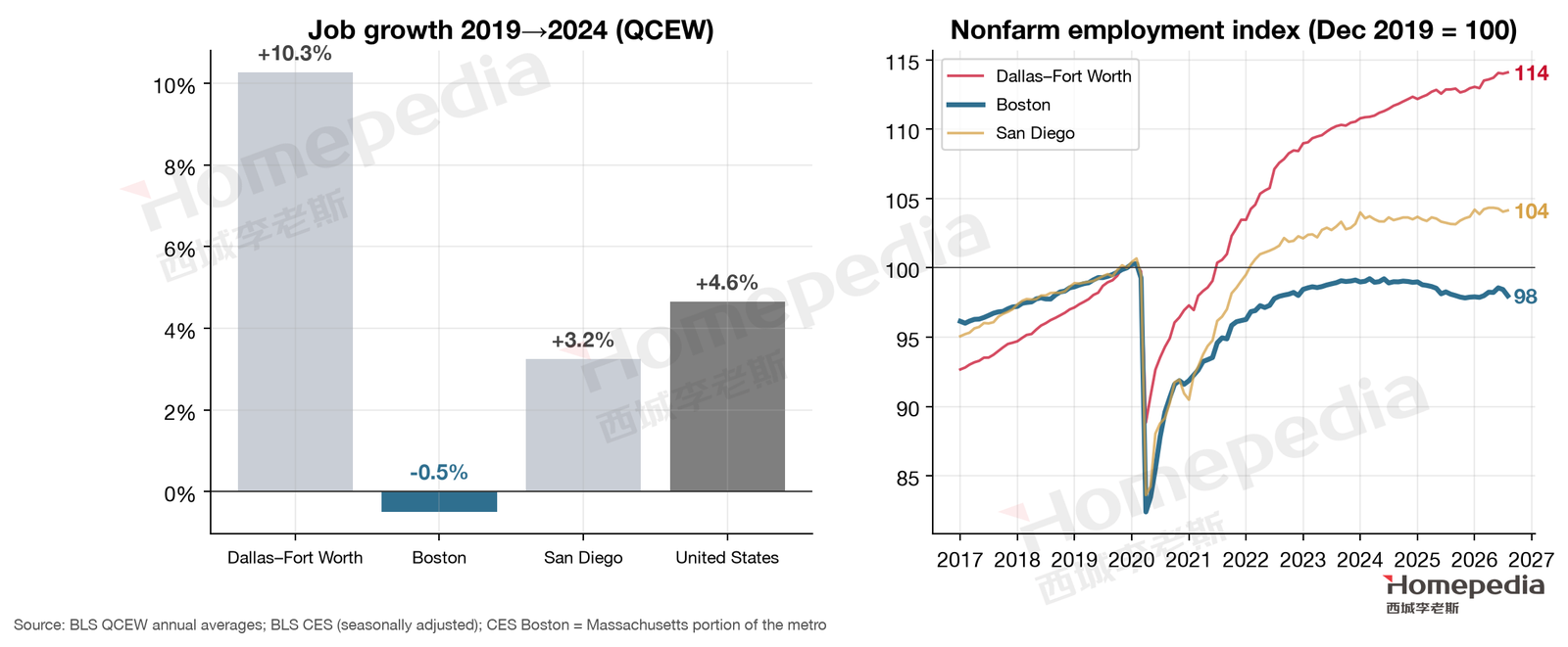
According to the BLS QCEW, average employment in the Boston metro fell from 2.722 million in 2019 to 2.708 million in 2024, a 0.5% decline; over the same period the U.S. grew 4.6%, San Diego 3.2% and Dallas 10.3% [1]. Monthly data show nonfarm employment in the Massachusetts portion of the metro at 2.732 million (seasonally adjusted) in August 2026, still 2.0% below December 2019 and essentially flat over the year (−0.1%) [2]. Boston is the only one of the three metros whose total employment has not returned to its pre-pandemic level.
Boston’s wages, however, are high and rising. Average annual pay across all industries rose from $82,092 in 2019 to $103,714 in 2024, up 26.3% [1]—in line with the nation, but about 37% higher in level. Boston’s problem is not low income but the lack of job growth: the existing high-income population can sustain high prices, but new buyers are limited.
2.2 Industry Composition
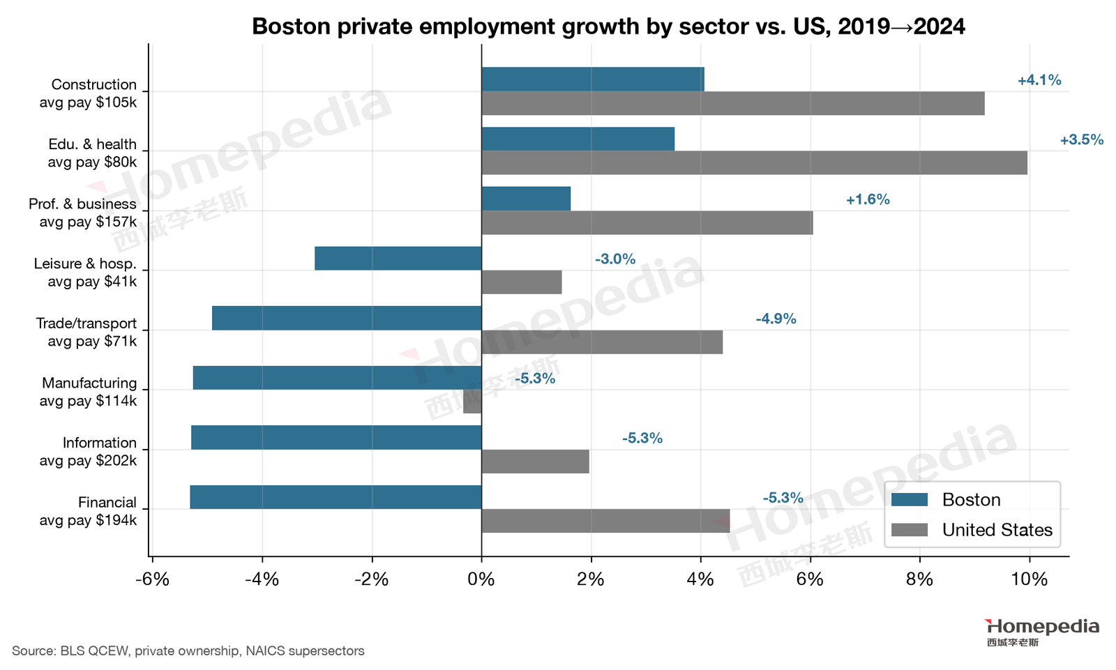
By sector (Figure 2), only three private industries grew in Boston from 2019 to 2024: education and health (+3.5%, about 587,000 jobs, vs. +10.0% nationally), construction (+4.1%) and professional and business services (+1.6%, about 523,000 jobs, average pay $157,291). Every other sector shrank: finance −5.3% (average pay $193,643), information −5.3% ($201,635), manufacturing −5.3% and trade/transportation −4.9% [1].
This is a classic high-pay knowledge economy: not many jobs, but very high pay per job. Boston’s professional and business services pay about 50% more than the same sector in Dallas, and finance about 60% more. That income level is what lets Boston maintain some of the highest home prices in the country without job growth.
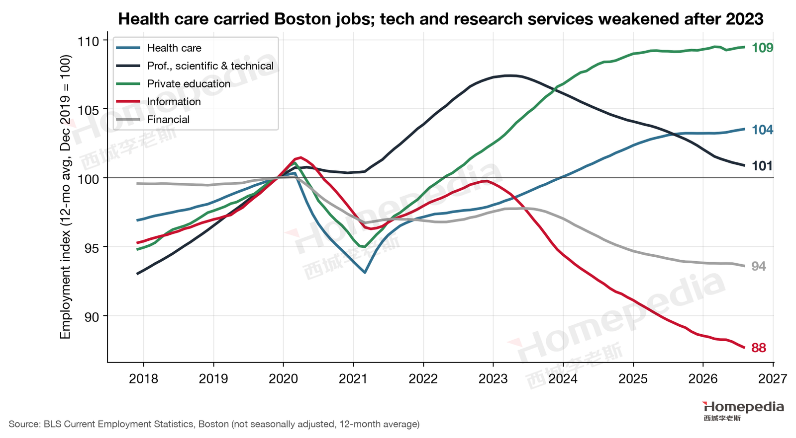
The monthly data (Figure 3) reveal the true source of resilience. As of August 2026, health care employment was 3.4% above late 2019, at about 469,000, the only large sector still growing; professional, scientific and technical services (including biotech R&D and consulting) were 0.9% below late 2019 and down 1.3% over the year; private education was 1.4% lower; information 14.8% lower; and finance 6.2% lower [2]. In other words, Boston’s knowledge-economy resilience has increasingly depended on the hospital system since 2023, while tech and research services weaken.
The hospital system works as ballast because its demand is largely immune to the business cycle. Greater Boston has several of the nation’s top teaching hospitals, whose revenue comes mainly from patient care—demand that does not disappear when rates rise or research funding falls, and that an aging population will keep increasing. As of August 2026, health care was about 17% of nonfarm employment in the Massachusetts portion of the metro [2]. These jobs span a wide range: physicians and research clinicians earning hundreds of thousands of dollars, and many mid-income nurses, technicians and administrators. The former support high-priced homes in suburban school districts; the latter support ordinary owner-occupied homes and rentals in gateway cities and the inner ring.
2.3 The Scale of High-Income Employment
Boston has the largest pool of high-income jobs of the three metros. Per OEWS 2025, occupations with mean pay of $150,000 or more account for about 320,000 jobs—more than 60% above Dallas (about 194,000), even though Boston’s total employment is only two-thirds of Dallas’s [3]. Management averages $174,356; life, physical and social scientists about $118,000; healthcare practitioners about $118,000.
This large stock of high earners explains Boston’s price floor: even without new buyers, existing affluent households trading up, upgrading and forming families generate enough demand to absorb roughly 10,000 new homes a year. It also explains the ceiling: when the number of high-income jobs stops growing, prices lose momentum for rapid gains.
3. Research Funding and Life Sciences: Source of Resilience and Risk
Boston–Cambridge is the world’s largest life-sciences cluster. The Massachusetts biopharma industry employed 113,503 people in 2025, and the state’s drug pipeline is 17.0% of the national total [4]. Harvard, MIT, Massachusetts General Hospital, Brigham and Women’s Hospital and others receive billions of dollars a year from the National Institutes of Health (NIH). This is the foundation of Boston’s high-income employment—and the largest source of uncertainty in 2025–2026.
3.1 Contracting Federal Research Funding
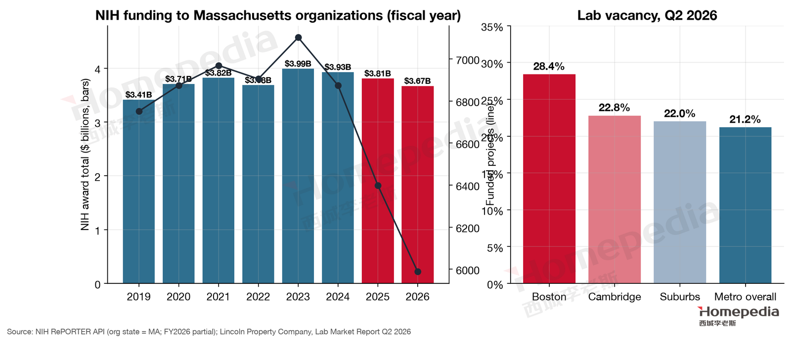
Using public NIH RePORTER data, we tallied NIH awards to Massachusetts organizations (Figure 4, left): a high of about $3.99 billion in FY2023, $3.93 billion in FY2024, $3.81 billion in FY2025 and $3.67 billion in FY2026 (data through early October), 6.6% below 2024; the number of funded projects fell from 6,874 in 2024 to 5,988 in 2026, down 12.9% [5].
Dollars fell less than project counts because awards canceled en masse in early 2025 were partly restored after litigation and settlements. GBH News, citing independent tracking data, reported that by June 2025 Massachusetts had lost 733 NIH grants with about $1.3 billion in unspent funds; including National Science Foundation (NSF) grants the total was about $2.6 billion, of which about $2.3 billion was at Harvard institutions [6]. Even with partial restoration, research institutions widely slowed hiring and expansion—the background to the weakening in professional, scientific and technical services in Figure 3.
3.2 Lab Oversupply and the First Biopharma Job Decline
The other side of life sciences is commercial real estate. Lincoln Property reports overall Greater Boston lab vacancy of 21.2% in Q2 2026—28.4% in Boston proper, 22.8% in Cambridge and 22.0% in the suburbs—with negative net absorption of 109,817 square feet in the quarter [7] (Figure 4, right). Labs built in large numbers during the pandemic met a funding squeeze, leaving severe oversupply.
On the employment side, the Massachusetts Biotechnology Council (MassBio) reports that Massachusetts biopharma employment fell 3.1% in 2025 to 113,503, the first annual decline in the more than two decades it has tracked the data [4]; only biomanufacturing bucked the trend, adding 238 jobs. The contraction was concentrated in R&D and early-stage companies while local production kept expanding; for housing, the core towns where researchers cluster, such as Cambridge and Somerville, are most affected.
3.3 Early Signs of Recovery
Capital markets have recovered ahead of jobs. MassBio reports that Massachusetts biopharma companies raised $3.45 billion of venture capital in the first half of 2026, up 25% year over year and a quarter of all U.S. biopharma VC, the strongest first half since 2023; eight Massachusetts companies went public, matching the total for 2024 and 2025 combined; and eleven companies were acquired for about $18.0 billion [4]. In the lab market, Cambridge showed signs of stabilization in Q2 2026, with Sanofi signing a roughly 900,000-square-foot lease in East Cambridge [7].
Some caution is warranted: a VC rebound first shows up as funding for a few leading companies, and it typically takes 6–12 months or longer to translate into broad hiring, while federal research funding still depends on policy. We treat a life-sciences recovery as the main trigger for the upside scenario, not a premise of the base case.
3.4 Implications for Housing
Research funding and life sciences affect housing through three channels:
- Slower growth in new high-income jobs. Researchers, postdocs and biotech engineers are important buyers of mid- to upper-priced homes in Cambridge, Somerville and Waltham. Slower hiring directly weakens owner-occupied demand there—consistent with the core’s lagging prices in §7.
- Fewer international students and researchers. Tighter visa policy and funding uncertainty have led some international graduate students and postdocs to delay or forgo coming to Boston (§8). They are mostly renters, so this weakens rental demand near campuses in the short run.
- The hospital system provides a floor. Unlike research funding, hospital clinical revenue comes mainly from Medicare, Medicaid and insurance payments, so employment is more stable. Continued growth in health care jobs is the key reason Boston’s demand has not fallen sharply.
We therefore read the map’s “Infrastructure upside: Med–high” this way: Boston has the nation’s best research and medical infrastructure, the source of long-run resilience; but in 2025–2026 that infrastructure is itself facing funding cuts, so its near-term boost to housing demand is limited.
4. Artificial Intelligence and the Labor Market: The Next Two Years
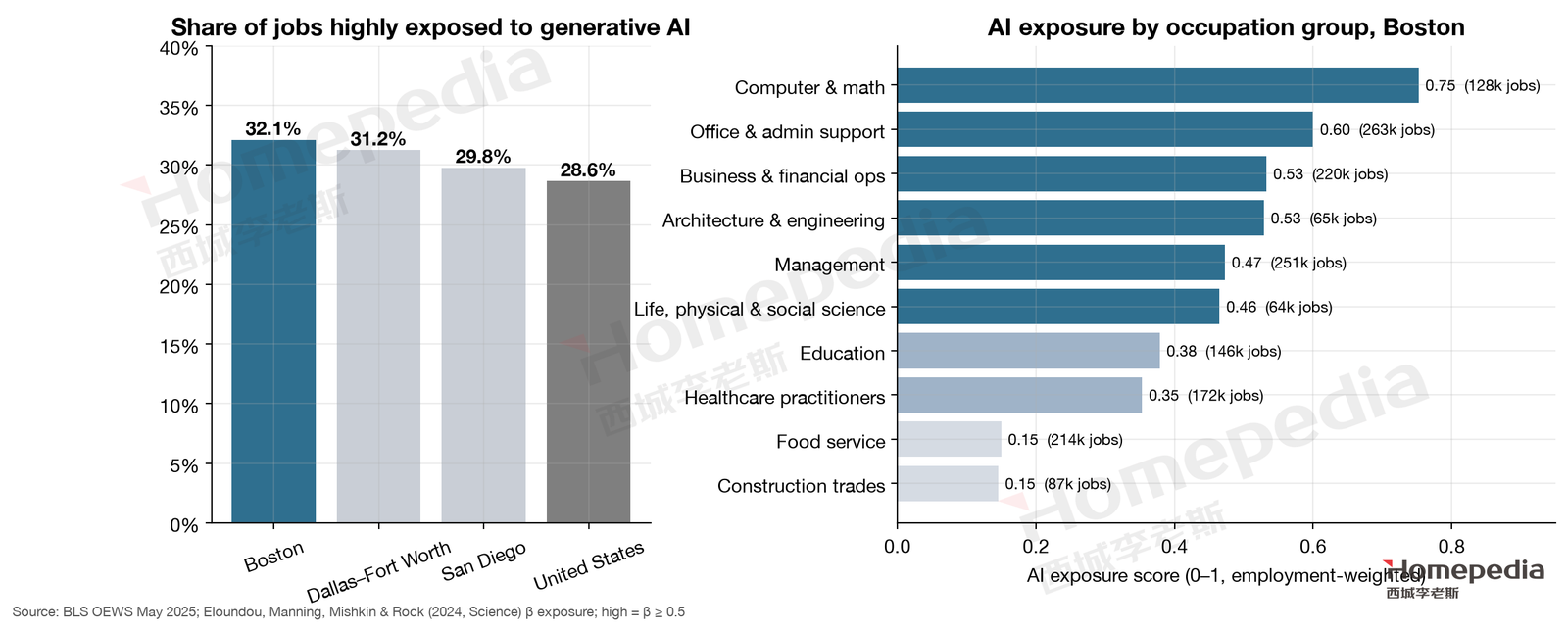
Following the method of Report No. 1, we matched BLS OEWS May 2025 occupational data with the occupational AI exposure scores of Eloundou et al. (2024, Science) [3][8]. In Boston, 32.1% of jobs—about 795,000—are highly exposed (score ≥ 0.5), the highest of the three metros, above Dallas (31.2%), San Diego (29.8%) and the U.S. (28.6%).
This is intuitive: the more white-collar and knowledge-intensive the metro, the more jobs are exposed to generative AI. In Boston, exposure is highest for computer and mathematical occupations (0.75, about 128,000 workers), office and administrative support (0.60, about 263,000), business and financial operations (0.53, about 220,000) and engineering (0.53, about 65,000); management (0.47, about 251,000) and life, physical and social science (0.47, about 64,000) are in the middle; healthcare practitioners (0.35, about 172,000) and education (0.38, about 146,000) are lower [3][8].
Exposure measures what the technology can do, not what will happen within two years. Over that horizon, AI’s effect on Boston’s housing demand is structural and concentrated at the entry point:
- Back-office and entry-level white-collar jobs come under pressure. Hiring for office administration, junior analysis and customer support will slow. A Dallas Fed study of Texas found postings for more automatable occupations fell about 8% relative to others [9]; similar Boston jobs likely face the same pressure. These workers are the main source of demand for core rentals and entry-level condos.
- The existing stock of high-income households will not shrink within two years. Tracking ADP payroll data, the Stanford Digital Economy Lab finds that AI’s employment effect so far has come almost entirely through reduced hiring of young workers; senior employees’ jobs have not yet been affected, and there have been no economy-wide layoffs [10]. Physicians, researchers, lawyers, senior engineers and managers remain employed, and they are the main buyers of single-family homes in suburban school districts. This is why high-end housing demand will not collapse within two years.
- AI is also a new Boston industry. Cambridge and Boston host many AI research groups and startups, and the combination of AI and life sciences (such as AI-driven drug discovery) is an important direction for the biotech recovery.
From a housing perspective, the most important AI effect in Boston over the next two years is its intersection with life sciences. More stages of drug development (target discovery, molecular design, clinical trial analysis) now use AI. That reduces the number of researchers each company needs, but it is also spawning a new wave of “AI + bio” companies. If the latter’s expansion outpaces the former’s contraction, high-income jobs in Cambridge and the Seaport will grow again and core owner-occupied demand will recover; if not, the core’s lag will last longer. This is one reason our two-year scenario analysis treats life-sciences hiring as the key turning signal.
The map’s “Medium” AI risk rating for Boston over two years is therefore consistent with the data: exposure is the highest of the three metros, but the effect so far is confined to hiring, and the net result is weaker rent-or-buy demand from entry-level white-collar workers in the core. It must be stressed that “Medium” holds only for two years. Boston’s 32.1% of highly exposed jobs are not evenly distributed; they are concentrated in the high-paying occupations that hold up prices. An occupation that hires no new entrants for ten years shrinks through retirement and attrition, and replacement is completed without layoffs. That process lies beyond this section’s horizon and is the subject of §10.
5. The Marginal Buyer: Migration, Income and Affordability
5.1 Persistent Domestic Out-Migration
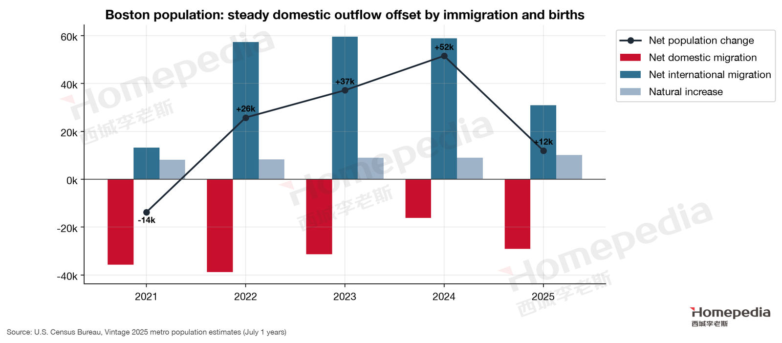
Census Vintage 2025 estimates show the Boston metro growing from 4.921 million in 2020 to 5.034 million in 2025, only about 110,000 people in five years [11]. Growth came entirely from immigration and natural increase: net domestic migration was negative every year in 2021–2025, between −16,000 and −39,000, and −29,132 in 2025; net international migration was about 58,000 a year in 2022–2024 and fell to 30,913 in 2025; natural increase was about 10,000 a year [11]. The pattern predates the pandemic: Boston lost about 104,000 residents to net domestic migration in 2011–2019.
The halving of international migration means Boston’s population growth slowed markedly in 2025—and international migrants, including graduate students, postdocs, physicians and engineers, are an important source of rental demand.
The housing implication is clear: Boston’s new residents are mainly international migrants, who almost all rent at first and only partly become buyers years later; those leaving are domestic households who have worked here for years and could have been buyers. Rental demand therefore benefits more from population flows than owner-occupied demand, while new owner-occupied buyers depend mainly on local income growth and family life cycles (marriage, children, trading up). This is the demographic basis of Wei Li’s judgment that core rentals are better supported than ordinary owner-occupied homes.
5.2 Departing Households Are Richer Than Arriving Ones
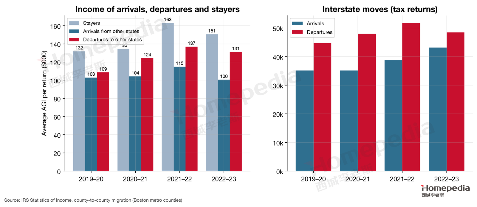
IRS county-to-county migration data reveal a fact that matters greatly for prices [12]. In tax year 2022–23, about 43,000 households moved into the Boston metro’s seven counties from other states, with average adjusted gross income of $101,000; about 48,000 households moved from those counties to other states, with average income of $131,000, 30% more than arrivals; households that stayed averaged $151,000 (Figure 7). In each of the last four tax years, departures outnumbered arrivals, and departing households earned more than arriving ones.
This is what the map means by “Marginal affluent buyer: Flat.” Many of those leaving are middle- and upper-middle-income households priced out of the homes they want in Boston, moving to New Hampshire, Maine or Southern metros; arrivals are mostly young students, researchers and early-career workers with lower incomes who mostly rent. The number of new affluent buyers is not growing; those buying in Boston are mainly affluent households already here.
5.3 Housing Affordability
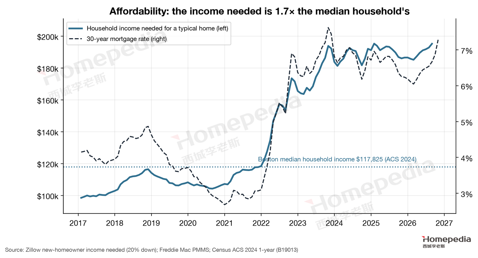
Zillow estimates that buying a typical Boston home with 20% down, keeping payments under 30% of income, required household income of about $195,229 in August 2026, versus $108,224 in December 2019 [13]. The metro’s median household income is $117,825 (2024 American Community Survey) [14]—the income needed is 1.66 times the median. Boston’s typical home value is 6.2 times median household income, far above Dallas (3.9×) and the U.S. (4.5×).
Box 1. Monthly Carrying Cost of a Typical Home
At Boston’s August 2026 typical value of $733,574, with 20% down (about $147,000), a loan of about $587,000 and a 7.28% 30-year fixed rate [15]:
- Principal and interest: about $4,015 a month
- Property tax (at an effective rate of 1.0%–1.3%; Boston’s FY2026 residential rate is $12.40 per $1,000 [16]): about $611–795 a month
- Homeowners insurance (assuming $2,000–3,000 a year): about $167–250 a month
- Total: roughly $4,800–5,060 a month (before condo fees and maintenance)
By comparison, a typical Boston single-family rental is about $3,648 a month and a typical home of any type about $3,073 [13]. At today’s rate, owning a typical home costs about $1,150–1,400 more per month in cash than renting a single-family home—plus a down payment of about $150,000.
Compare late 2019: the same home was worth about $498,000, the average rate was 3.72%, and principal and interest was about $1,838 a month. Prices rose 47%, but the payment rose to 2.2 times its earlier level. The “rent beats buy” gap is far larger in Boston than in Dallas—the fundamental reason rental demand is firm.
5.4 Rate Lock-In: New Listings at 80% of Pre-Pandemic
Affordability constraints affect sellers as well as buyers. Realtor.com data show that over the past 12 months, new listings in the Boston metro averaged only 79% of the same months in 2017–2019, versus 96% in Dallas [17]. Many owners bought or refinanced at around 3% in 2020–2022; selling now means borrowing again at over 7%, which could double their payment. So they don’t sell.
This rate lock-in has two consequences: resale supply shrinks further on top of already minimal new construction, keeping inventory below pre-pandemic levels; and sales volume stays depressed—those who can’t afford to buy can’t get in, and those who can afford it won’t trade. That is the real meaning of the map’s “supply limits support prices while affordability keeps volume muted”: prices don’t fall, but liquidity is poor. For households that must sell, good homes still sell easily; for buyers waiting for a price drop, that strategy rarely works in Boston.
6. Housing Supply Constraints and Price Resilience
Box 2. Why Boston Cannot Build
Boston’s supply constraints operate on two levels. The first is geography: the Atlantic, the harbor, the Charles River and wetlands fragment developable land, and the city and inner-ring towns are long since built out. The second is institutions: housing development in Massachusetts is governed largely by the zoning of 351 individual cities and towns; many suburbs have long allowed only single-family homes, multifamily housing requires special permits, and residents can delay or block projects at public hearings. Glaeser and Ward’s study of 187 Greater Boston towns found that local land-use rules substantially reduced new construction and are an important cause of the region’s high prices [18].
Massachusetts is trying to change this. The MBTA Communities Act, passed in 2021, requires 177 cities and towns served by commuter rail and transit to designate at least one district where multifamily housing is allowed as of right. As of January 2026, 133 communities were compliant; but a Boston Foundation review found the law had so far pushed only about 7,000 homes into the permitting and development pipeline, fewer than a third within half a mile of transit—gains that are “real but modest” [19].
6.1 Scale of New Housing Supply
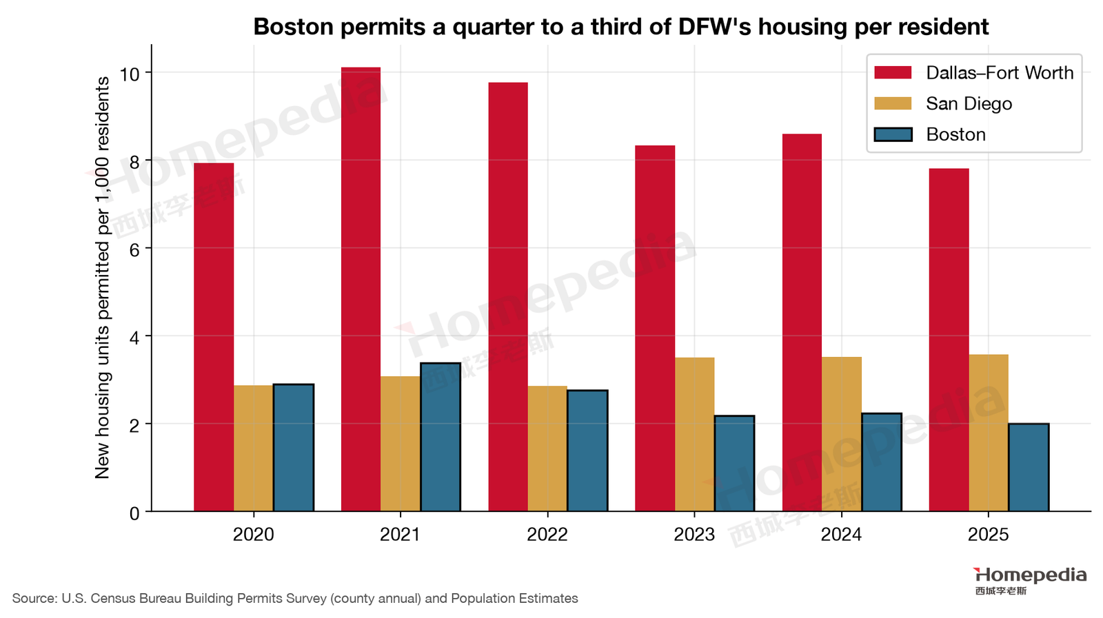
Census building permit data show the Boston metro’s seven counties permitted 76,574 homes in 2020–2025, 68% of them multifamily [20]; Dallas permitted 423,000 over the same period. Per capita (Figure 9), Boston permits 2.0–3.4 homes per 1,000 residents a year, on a downward trend: in 2025 it permitted only 2.0 per 1,000, or 10,072 homes, the lowest in six years. Dallas permitted 7.8 per 1,000 the same year.
6.2 Supply Elasticity and Long-Run Prices
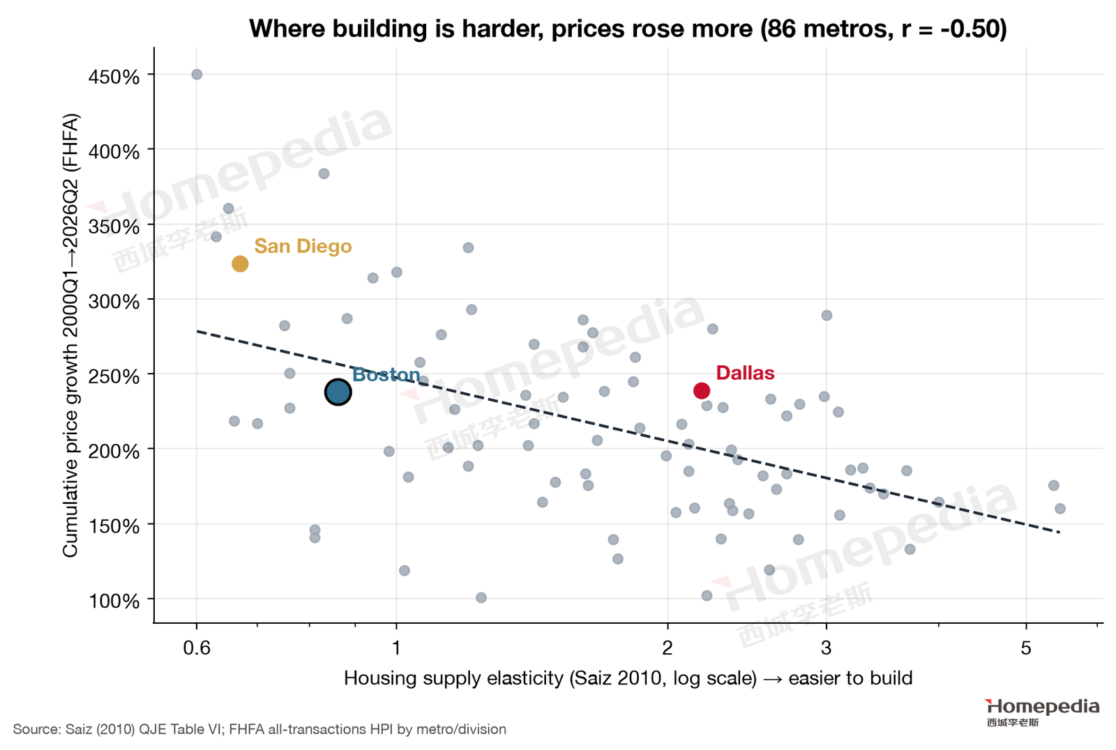
Saiz (2010) estimates Boston’s long-run housing supply elasticity at 0.86, the 15th lowest of 95 metros (1 = hardest to build), versus 2.18 for Dallas and 2.80 for Fort Worth [21]. Across 86 matched metros, lower elasticity goes with larger price gains since 2000 (correlation −0.50, Figure 10) [21][22].
Notably, Boston’s cumulative gain since 2000 (+238%) sits near the trend line and roughly matches Dallas (+239%). The two metros reached similar outcomes by entirely different routes: Dallas through strong demand growth, Boston through extremely constrained supply. Dallas’s gains get caught up by new supply; Boston’s get “locked in.”
6.3 Flat Demand, Rising Prices
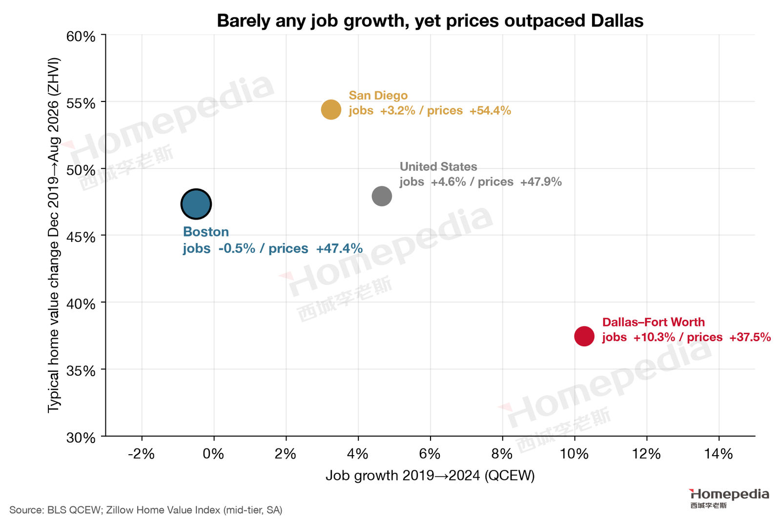
Put demand and prices together (Figure 11) and Boston stands out: it had the lowest job growth of the four areas compared (−0.5%), yet its price gain (+47.4%) exceeds Dallas (+37.5%) and matches the U.S. (+47.9%). Through December 2024 alone, Boston rose 44.0%, close to Dallas (45.7%) and the U.S. (46.9%)—itself a sign of supply constraint given near-zero job growth. After 2025, Dallas turned down while Boston kept rising, and the gap widened quickly.
How does a metro with no job growth see prices rise 47%? Three factors worked together:
- Income growth. The number of jobs didn’t grow, but pay rose sharply: average annual pay rose 26.3% in five years to more than $103,000 in 2024 [1]. Buying power depends on total income, not just headcount.
- Near-zero supply. Only about 10,000 homes are added each year in a metro of about 2 million households; even without demand growth, normal household formation (young adults leaving home, divorce, older adults living alone) is enough to absorb that.
- Rate lock-in reduced resale supply. As §5 shows, new listings are only 80% of pre-pandemic, deepening the scarcity of homes for sale.
All three were present in 2019–2024, which is why Boston’s prices rose despite stagnant demand. But each has limits: income growth depends on the health of high-pay industries, and finance, information and research services are contracting; lock-in will gradually loosen over time and as rates fall.
6.4 Sensitivity of Prices to Demand
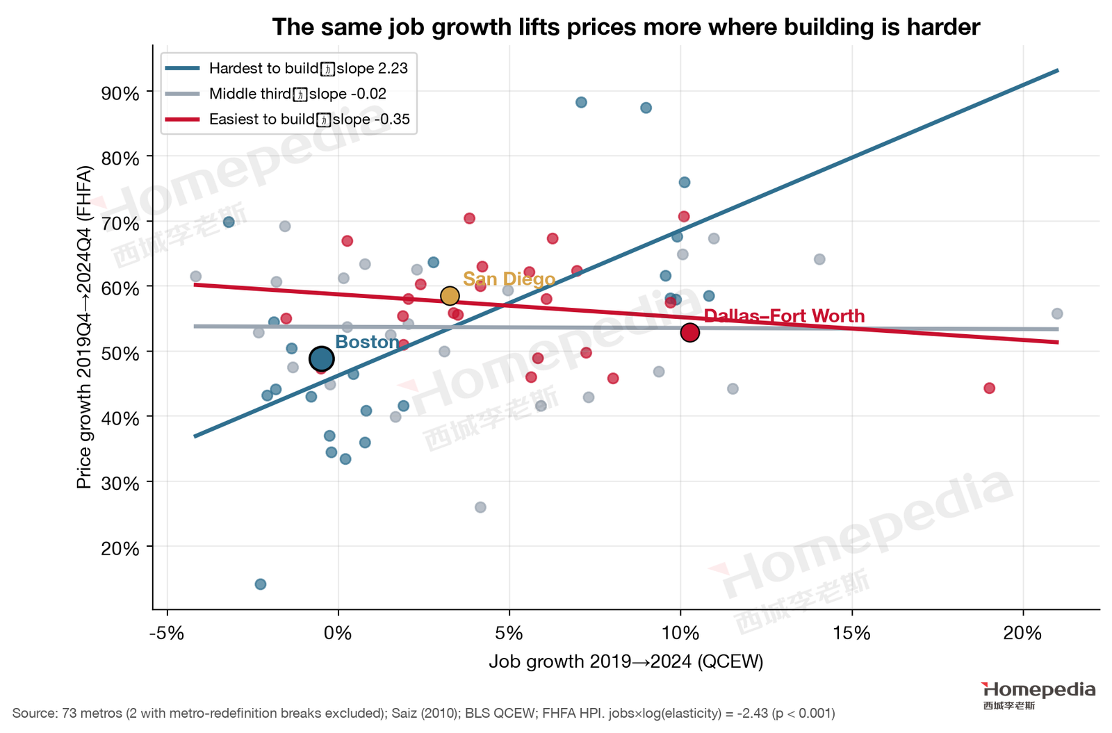
In Report No. 1 we ran a 73-metro regression of price growth on job growth, supply elasticity and their interaction; the interaction coefficient was −2.43 (p < 0.001) [1][21][22]. Plugging in Boston’s elasticity (0.86), the model implies that each percentage point of job growth raises Boston prices by about 2.3 points, versus roughly zero in Dallas (Figure 12).
This cuts both ways:
- On the way up, any recovery in demand—a life-sciences funding rebound, restored research funding, lower rates—passes through to prices at more than twice the magnitude. This is why Boston’s prices have been strong over the long run.
- On the way down, a contraction in demand is amplified just the same. If research funding and white-collar employment keep shrinking, Boston’s price adjustment will exceed the change in jobs. Over two years, this is why we treat federal research funding as the largest risk; over ten, it is why the consequences of AI replacing judgment jobs would land on prices at more than twice their magnitude (§10).
With near-zero job growth in 2019–2024, the “amplifier” was not triggered; Boston’s gains came mainly from income growth, demand pulled forward by ultra-low rates, and persistent undersupply.

7. Price Structure: Where It Is Strong, Where It Is Weak
7.1 Aggregate Price Trends
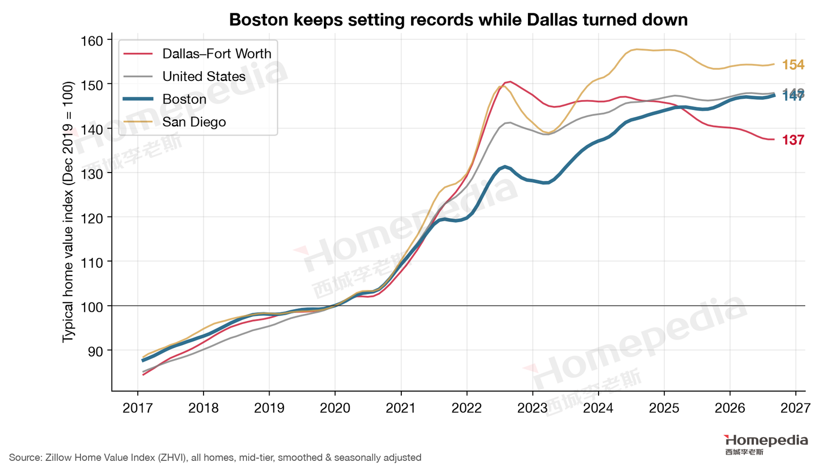
The Zillow Home Value Index shows Boston’s typical value at $733,574 in August 2026, a new record, 47.4% above late 2019 and up 2.1% over the year [13]. Unlike Dallas (8.6% below peak) and San Diego (2.1% below peak), Boston only briefly corrected during the rapid rate increases of 2022–2023 and has risen steadily since (Figure 14). FHFA’s repeat-sales index likewise shows the Boston division 58.4% above 2019Q4 as of 2026Q2 [22].
7.2 Inventory and Seller Bargaining Power
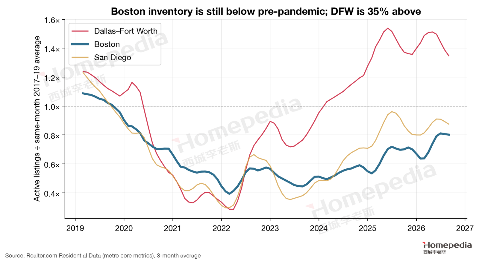
Realtor.com data show 9,017 active listings in the Boston metro in September 2026, only about 80% of the 2017–2019 average for the same months (Figure 15) [17]. Notably, inventory is up 16.1% from a year earlier—with rates higher and the economy weaker, inventory is slowly recovering, but it remains well below pre-pandemic levels.
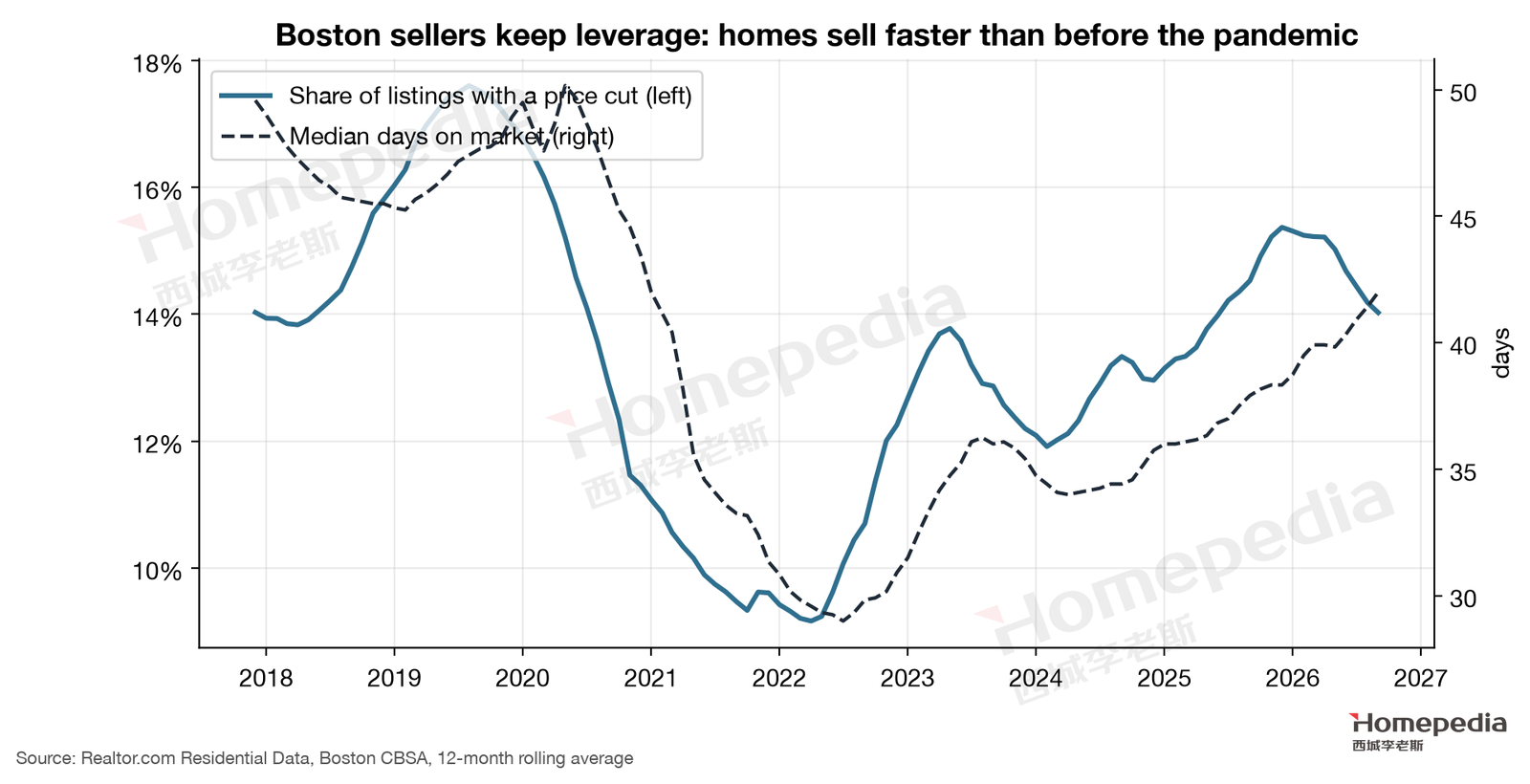
Sellers still have the upper hand (Figure 16). In September 2026, 16.6% of Boston listings had a price cut, slightly above the 2017–2019 average of 15.6%; the median listing had been on the market 43 days, shorter than the pre-pandemic average of 48 days [17]. Of the three metros, Boston is the only one where homes sell faster than before the pandemic.
7.3 Price Tiers: Almost No Divergence
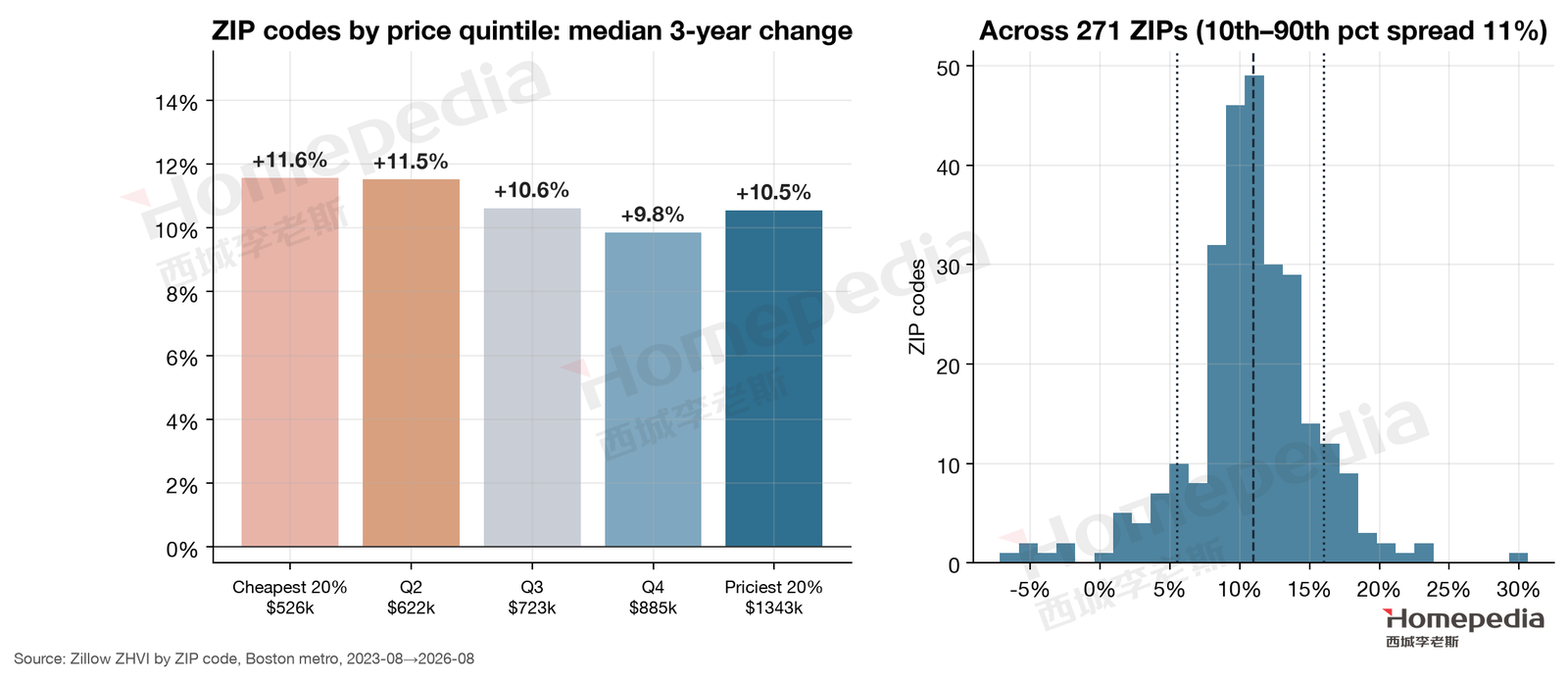
In sharp contrast with Dallas’s “cheap homes fell, expensive homes held,” Boston’s 271 ZIP codes rose almost in lockstep across price tiers (Figure 17). From August 2023 to August 2026, the cheapest fifth (median about $526,000) rose 11.6% and the most expensive fifth (median about $1.34 million) 10.5%, with the middle groups between 9.9% and 11.5%; the 10th-percentile ZIP rose 5.5% and the 90th-percentile 16.0% [13]. Since 2019, cheaper ZIPs actually rose the most (+60.0%) and the priciest 53.2%.
This is typical of a supply-constrained market: the shortage is comprehensive, homes in every tier are scarce, and prices rise together. Boston’s divergence lies not between price tiers but between places and products.
Compared with Report No. 1, the fundamental difference between the two markets is clear. In Dallas, builders’ new homes concentrate in the $250,000–$400,000 band, so new supply presses directly on the low end: the cheapest ZIPs fell most and the priciest held best. In Boston, there is no large-scale new supply to hold down any tier, so all tiers rise; what determines gains is who is buying and what they are buying. Middle-income households priced out of the core pour into gateway cities, lifting the low end there; while the core’s buyer base (life sciences, tech, academia) is precisely the group that is shrinking, and the core’s condo-heavy product doesn’t match post-pandemic buyers’ preference for space.
7.4 Geographic Divergence: The Core Lags, the Suburbs Lead
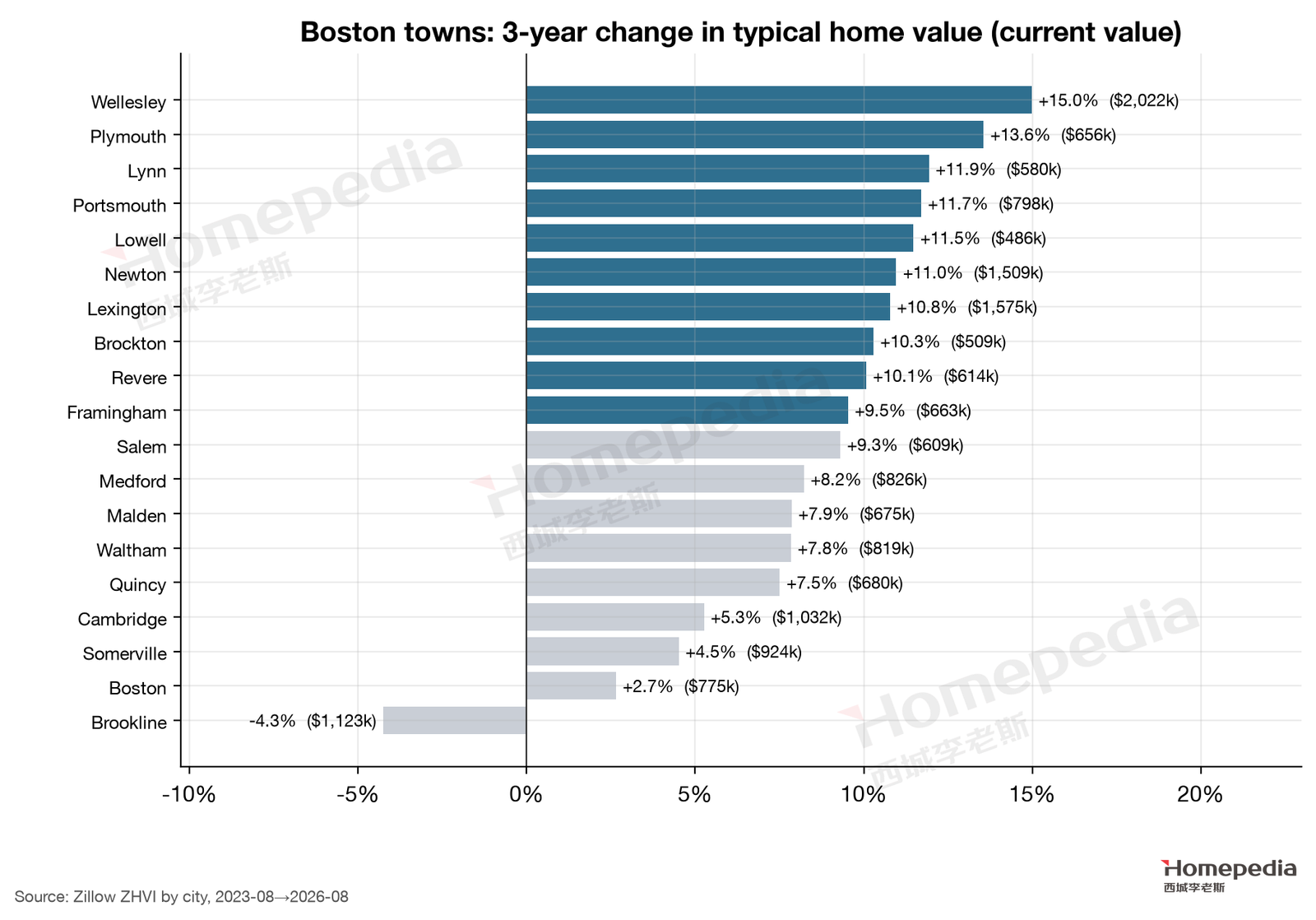
Town-level data reveal Boston’s most important structural shift (Figure 18). The largest three-year gains are in suburbs and gateway cities: Wellesley +15.0%, Plymouth +13.6%, Lynn +11.9%, Portsmouth (NH) +11.7%, Lowell +11.5%, Newton +11.0%, Lexington +10.8%. The smallest are in the core: Brookline −4.3%, Boston proper +2.7%, Somerville +4.5%, Cambridge +5.3% [13].
Over the longer window since late 2019, the gap is striking: Lowell +59.3%, Plymouth +64.6%, Wellesley +60.6%; but Boston proper only +15.9%, Cambridge +14.3% and Brookline +7.0% [13].
The core lags for three reasons: product mix—the core is dominated by condos and older multifamily buildings, while post-pandemic buyers prefer single-family homes with space; buyer mix—core buyers come heavily from life sciences, tech and academia, the groups contracting most since 2023; and starting price—core prices were already high, so affordability constraints bit there first.
7.5 Property Type: Condos Underperform
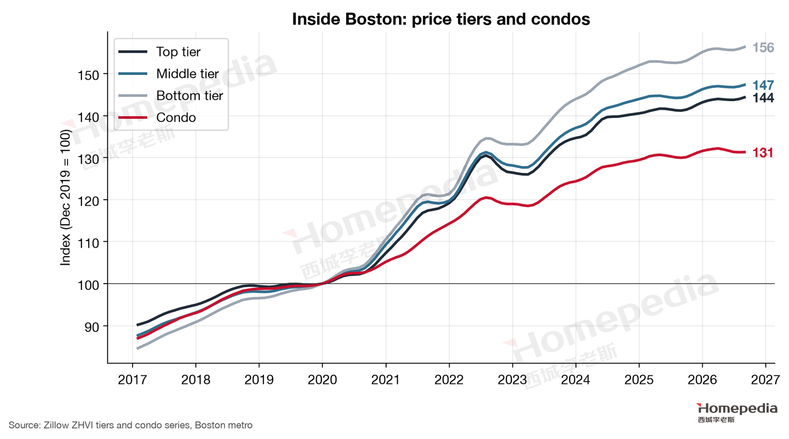
Zillow’s tiered indexes (Figure 19) show Boston’s bottom tier up 56.4% since late 2019, the middle tier 47.4% and the top tier 44.4%, all at record highs; condos are up only 31.3%, 0.7% below their March 2026 peak and up just 1.0% over the year, at a typical $582,443 [13]. Condos underperform for the same reasons the core lags, plus rising maintenance costs, special assessments and insurance in older buildings. The map’s condo view is “split: transit cores hold; aging-building costs are a risk”—the data support the second half, while the first half must be judged building by building: newer, financially healthy buildings near major transit (such as the Red and Orange Lines) clearly outperform older ones.
8. The Rental Market: Why Core Rentals Are Better Supported
8.1 The Core: Rents Rose About Twice as Fast as Home Values
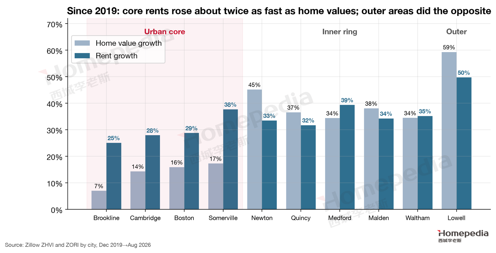
This section is the most direct test of Wei Li’s judgment. We placed Zillow’s town-level home value and rent indexes side by side and compared growth since late 2019 (Figure 20) [13]:
| Town | Ring | Home value growth | Rent growth |
|---|---|---|---|
| Brookline | Core | +7.0% | +25.1% |
| Cambridge | Core | +14.3% | +27.9% |
| Boston proper | Core | +15.9% | +28.8% |
| Somerville | Core | +17.3% | +37.7% |
| Medford | Inner ring | +34.4% | +39.4% |
| Waltham | Inner ring | +34.5% | +35.2% |
| Quincy | Inner ring | +36.6% | +31.7% |
| Newton | Inner ring | +45.2% | +33.5% |
| Lowell | Outer | +59.3% | +49.7% |
The pattern is clear: in the core, rents rose about twice as fast as home values; in outer areas, home values outpaced rents. That is what “core rentals are better supported than ordinary owner-occupied homes” means: demand to live in the core is still strong—students, young professionals and hospital and university staff need to be there—but they increasingly rent rather than buy, because the bar to ownership is too high and the core’s (largely condo) product is losing appeal.
8.2 Overall Rent Trends and Rent Burden
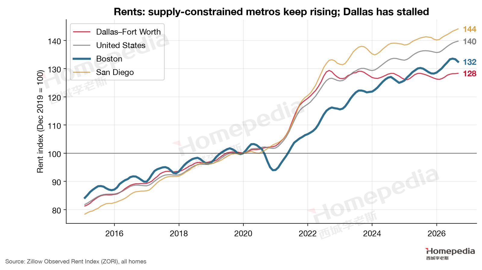
Metro-wide (Figure 21), Boston’s typical rent is $3,073, 32.4% above late 2019 and up 2.4% over the year; single-family rents are up 41.2% (about $3,648) and apartment rents 31.5% (about $3,035) [13]. Boston’s long-run rent growth is below San Diego (44.1%) and the U.S. (39.7%) but above Dallas (28.3%)—achieved without population growth.
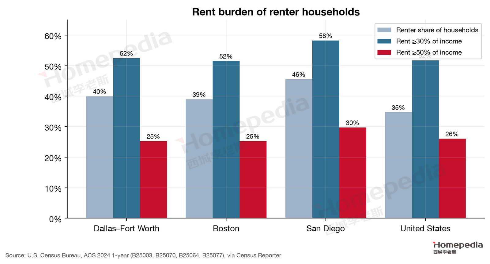
The American Community Survey shows 39.0% of Boston metro households rent, above the national 34.7%; 51.5% of renter households pay more than 30% of income in rent and 25.3% more than half (Figure 22) [14]. Median rent is $2,093 and median home value $681,100, both among the highest of U.S. metros.
8.3 Short-Term Pressures: Students and New Supply
Boston’s rental market also faced some short-term pressure in 2025–2026:
- Fewer international students. In fall 2025, new international enrollment nationwide fell about 17%; in Boston, international graduate students at Boston University fell about 10%, international students at UMass Boston about 17%, and Northeastern had 538 fewer; vacancies rose in student neighborhoods around Northeastern and Mission Hill [23]. Boston proper has about 152,000 college students [24], so student demand matters greatly for the core rental market.
- New deliveries and rising vacancy. Colliers reports Greater Boston multifamily vacancy of 6.9% in Q1 2026, up 0.8 points year over year [25]; Matthews reports average asking rent of $3,010 in August 2026, up 2.0% [26].
These pressures are cyclical and do not change the structural support for core rental demand.
8.4 Who Rents, and Why They Don’t Buy
Putting the data together sketches the structure of Boston’s rental demand. The first group is students and young researchers: about 150,000 college students in the city plus many postdocs and residents, highly mobile, almost all renting, concentrated in the core. The second is professionals with good incomes who still can’t buy: a typical home requires about $195,000 of household income, and a dual-income couple earning $150,000 combined—upper-middle-income in Boston—still falls short and keeps renting. The third is city dwellers who choose to rent: in the core, renting an apartment costs over $1,000 a month less than owning a comparable home, without the risk of major repairs in an older condo building, so renting is the more rational financial choice.
What these groups share is that they need to live in or near the core but cannot or will not buy at current prices. As long as core employment (hospitals, universities, life sciences) remains, their rental demand will not disappear—the fundamental reason core rents keep outpacing home values.
8.5 Policy: Rent Control on Hold
On June 23, 2026, the Massachusetts Supreme Judicial Court unanimously ruled that a statewide rent-control ballot initiative could not appear on the November 2026 ballot because it impermissibly related to religious institutions [27]. The proposal would have capped annual rent increases on most rental units at the lower of inflation or 5%; earlier polls showed about 60% of voters in support [27]. The state’s 1994 ban on rent control therefore remains in force at least through 2026, reducing near-term policy risk for rental investors—but the level of public support suggests the issue will likely return.
9. Comparative Analysis: Dallas–Fort Worth, Boston and San Diego
| Indicator | Dallas–Fort Worth | Boston | San Diego | Source |
|---|---|---|---|---|
| Job growth 2019→2024 | +10.3% | −0.5% | +3.2% | BLS QCEW [1] |
| Net domestic migration (2025) | +18,197 | −29,132 | −23,876 | Census [11] |
| Median household income (2024) | $92,733 | $117,825 | $109,132 | ACS [14] |
| Typical home value (Aug 2026) | $360,437 | $733,574 | $930,785 | Zillow [13] |
| Home value ÷ median income | 3.9× | 6.2× | 8.5× | Computed |
| Price change Dec 2019→Aug 2026 | +37.5% | +47.4% | +54.4% | Zillow [13] |
| Distance from recent peak | −8.6% | 0.0% (record) | −2.1% | Zillow [13] |
| Permits per 1,000 residents (2025) | 7.8 | 2.0 | 3.6 | Census BPS [20] |
| Active listings ÷ pre-pandemic | ~1.35× | ~0.80× | ~0.88× | Realtor.com [17] |
| Supply elasticity (Saiz 2010) | 2.18 / 2.80 | 0.86 | 0.67 | Saiz [21] |
| Share of jobs highly exposed to AI | 31.2% | 32.1% | 29.8% | OEWS × Eloundou et al. [3][8] |
| Jobs in occupations paying $150k+ | ~194,000 | ~320,000 | ~111,000 | OEWS [3] |
| Share of payroll in occupations paying $150k+ | 13.5% | 27.0% | 18.8% | OEWS × mean wage [3] (§10) |
The three metros represent three housing markets: Dallas is “strongest demand, even stronger supply,” Boston is “flat demand, minimal supply,” and San Diego is “scarce but fragile.” Boston is distinctive in sustaining the second-largest price gain of the three with the weakest demand growth, relying on some of the most constrained supply in the country and the largest stock of high earners.
For investors, the most important implication is that the sources of risk are entirely different. Dallas’s risk is oversupply, so avoid new-construction-heavy exurbs and choose established neighborhoods new homes can’t replicate; Boston’s risk is a demand shock—supply will almost never be the problem—so watch research funding, life-sciences financing and white-collar employment; San Diego’s risk is affordability and the fragility of affluent buyers. The same strategy of “buy single-family homes in established neighborhoods” rests on entirely different reasons in each metro.
10. The Next Ten Years: Artificial Intelligence and Judgment Jobs
The conclusions of the first nine sections rest on one premise: the high-income households that hold up Boston’s prices will stay. Over two years that premise broadly holds; as §4 showed, AI’s effect on employment so far is confined to slower hiring and entry-level jobs and has not reached the existing stock of high earners. Ten years is a different matter. Wei Li’s long-run judgment on Boston is: over the next ten years, AI will take away most of the jobs that depend on judgment, and Boston home prices are very likely to fall substantially. This section tests that judgment in three steps: first, how much of the income pool that supports prices is exposed to AI; second, how prices behaved the last time Boston lost a high-paying industry (1988–1995); third, a ten-year projection by two methods. One caveat comes first: the numbers in this section are projections, not forecasts. Replacement rates, amplification multiples and timing are all extrapolated from existing data and literature, and the uncertainty is far larger than in the preceding sections.
10.1 The Income Pool Behind Prices: Who Buys a $730,000 Home
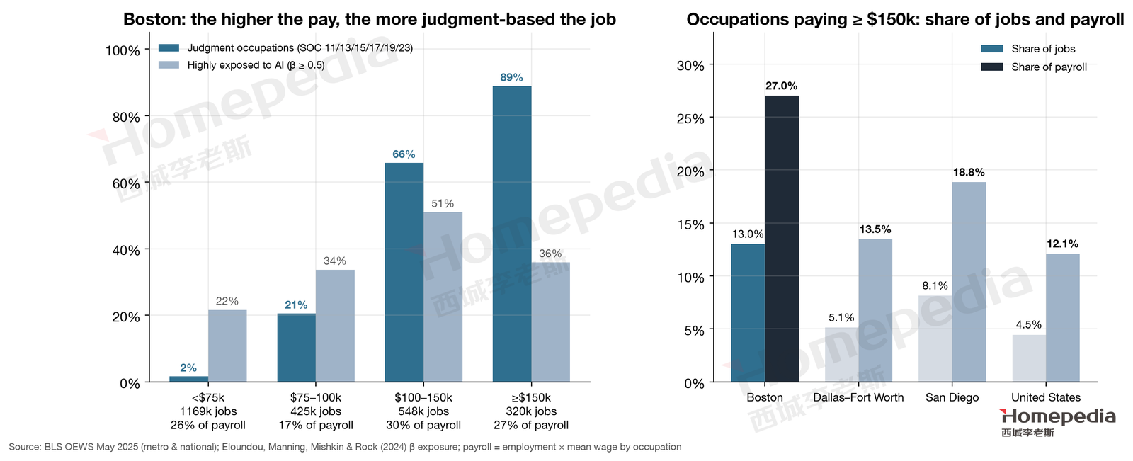
§5 showed that buying a typical home with 20% down requires household income of about $195,000. That threshold confines Boston’s buyers to a narrow group. We sorted OEWS 2025 occupations into four bands by mean annual pay and split each band by Eloundou et al.’s (2024) exposure score and by major occupational group (Figure 23, left) [3][8]:
| Occupational mean pay | Jobs | Share of metro payroll | In judgment occupational groups | Highly exposed to AI (β ≥ 0.5) |
|---|---|---|---|---|
| Under $75,000 | 1,169,000 | 26% | 2% | 22% |
| $75,000–100,000 | 425,000 | 17% | 21% | 34% |
| $100,000–150,000 | 548,000 | 30% | 66% | 51% |
| $150,000 and above | 320,000 | 27% | 89% | 36% |
“Judgment occupational groups” means six SOC major groups: management (11), business and financial operations (13), computer and mathematical (15), architecture and engineering (17), life, physical and social science (19) and legal (23). Their core work is analysis, decision-making, design, writing and advice. In Boston these six groups hold about 750,000 jobs, 30.5% of employment but 47.7% of payroll, with an employment-weighted AI exposure of 0.54; by comparison, healthcare practitioners score 0.35, education 0.38 and construction 0.15 [3][8].
Of the 320,000 jobs paying $150,000 or more, 284,000 (88.8%) fall in these six groups: management 199,000 (including 71,000 general and operations managers, 22,000 financial managers and 21,000 computer and information systems managers), computer and mathematical 57,000 (42,000 software developers) and legal 21,000; healthcare practitioners account for only 25,000 (7.7%) and education 11,000. The wages of these 284,000 judgment jobs sum to 23.7% of the entire metro payroll. Combining the two bands at $100,000 and above, the main source of dual-income households that reach the $195,000 threshold, gives 867,000 jobs and 57% of payroll, 74% of them in judgment groups.
Figure 23 (left) also shows something that needs explaining: the “highly exposed” share in the $150,000-plus band (36%) is lower than in the $100,000–150,000 band (51%). The reason is that management occupations score 0.48, just under the 0.5 threshold. The score measures the share of an occupation’s tasks for which a 2023-era large language model with tools could halve the time required, and the coordinating, negotiating and accountability parts of management were rated hard to replace at the time. On a ten-year horizon the threshold means little. Capabilities change: the scores were built with GPT-4-generation models, and reasoning, coding and autonomous multi-step execution have advanced markedly in the two years since. And the number of managers depends on the number of people managed; if analysts, engineers and lawyers become fewer, managers will not stay as numerous. For the ten-year question, “judgment occupational group” is therefore a better denominator than “β ≥ 0.5”, and the scenarios below use it.
Against other metros (Figure 23, right), Boston’s dependence on this group is in the highest tier nationally: occupations paying $150,000 or more are 13.0% of all jobs and 27.0% of payroll, versus 5.1% and 13.5% in Dallas, 4.5% and 12.1% nationally, and 8.1% and 18.8% in San Diego. In other words, twice the national share of Boston’s price base rests on high-paying judgment jobs. Health care and education (SOC 25, 29 and 31), widely regarded as the least exposed to AI, hold 374,000 Boston jobs and 16.6% of payroll, but only 36,000 of those jobs pay $150,000 or more. They can support ordinary owner-occupied homes and rentals in the gateway cities and the inner ring; they cannot support prices in the core and the top school districts.
10.2 Replacement Rates: The Literature and the Last Two Years
No one can prove with data how many judgment jobs AI will replace within ten years. What we can do is lay out the main institutional and academic estimates and set them against what has already happened in the past two years.
| Source | Estimate | Horizon |
|---|---|---|
| Eloundou et al. (2024, Science) [8] | About 19% of U.S. workers have at least half their tasks exposed to large language models | None (capability assessment) |
| Goldman Sachs (Briggs & Kodnani, 2023) [28] | About two-thirds of U.S. and European occupations partly exposed; about a quarter of current work could be substituted; about 7% of U.S. workers could be replaced and 63% complemented | 10 years |
| IMF (Cazzaniga et al., 2024) [29] | About 60% of jobs in advanced economies exposed; roughly half of those may benefit, the other half face replacement or lower pay | None |
| McKinsey Global Institute (2023) [30] | 29.5% of U.S. work hours could be automated by 2030 (21.5% without generative AI); 30% for business and legal professionals | To 2030 |
| Acemoglu (2024) [31] | Only about 4.6% of tasks can be profitably automated; total factor productivity gain of no more than 0.66% over ten years | 10 years |
| World Economic Forum (2025) [32] | 170 million jobs created and 92 million displaced globally by 2030, a net gain of 78 million | To 2030 |
The range is wide. At one end is Acemoglu’s “almost no effect”; at the other, from the standpoint of replacement, is the IMF’s “half of exposed jobs in advanced economies face replacement,” which works out to about 30% of all jobs. Wei Li’s “most taken away” corresponds roughly to the IMF’s upper bound and to McKinsey’s estimate for business and legal occupations (30% of work hours).
More persuasive than estimates is what has already happened. Using ADP payroll data, the Stanford Digital Economy Lab found that employment of 22- to 25-year-olds in the occupations most exposed to AI (software development, customer service and the like) was 13% lower in August 2025, relative to their peers in unexposed occupations; the study revised the gap to 16% in November 2025 and to 19% in August 2026, and reports that it has “widened continuously since first recorded.” The adjustment has come mainly through reduced hiring rather than layoffs, and senior employees’ jobs have not yet been affected [10]. The Dallas Fed found job postings in highly automatable occupations down about 8% relative to others [9]. Boston’s own data agree: as of August 2026, information employment was 14.8% below late 2019, finance 6.2% below, and professional, scientific and technical services down 1.3% over the year (§2).
Two things follow. First, the institutional estimates made in 2023 used the model capabilities of the time, and the labor market’s actual response, at least at the entry point, has been faster than those estimates implied. Second, the effect so far is concentrated among young and entry-level workers, which is exactly why §4 finds the two-year effect limited; but an occupation that hires no new entrants for ten years shrinks through retirement and attrition, and replacement is completed without mass layoffs. Ten years is precisely the horizon on which that process operates.
10.3 Precedent: Boston and Hartford, 1988–1995
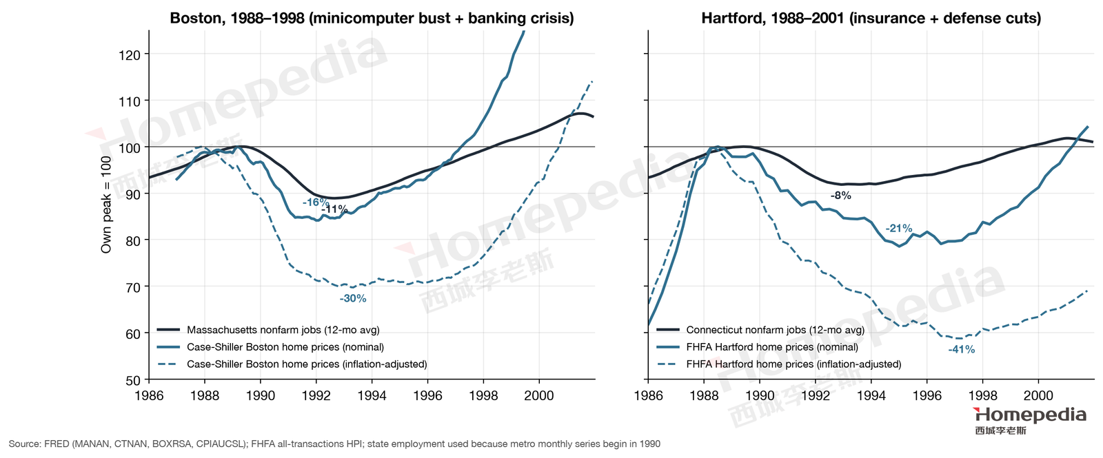
Boston has faced the loss of a high-paying industry before. The “Massachusetts Miracle” of the 1980s was built on the minicomputer industry (DEC, Wang, Data General, Prime), defense contracts and post-deregulation bank expansion; after the summer of 1987 all three turned at once. Case (2000) recounts that employment had begun falling by the 1988 election and kept falling until the end of 1991, “losing more than 360,000 jobs from a peak of 3.2 million, more than 11.5% of nonfarm employment”; the Bank of New England, with $32 billion in assets, was closed by the FDIC in January 1991, with more than 90% of its losses from real estate loans [33]. We re-examined this episode with the original FRED and FHFA series (Figure 24, left) [34][22]:
| Series | Peak | Trough | Decline | Regained peak |
|---|---|---|---|---|
| Massachusetts nonfarm employment (12-month average) | June 1989 | September 1992 | −11.1% | May 1998 (8.9 years) |
| Case-Shiller Boston home prices (nominal) | March 1989 | January 1992 | −15.9% | April 1997 (8.1 years) |
| FHFA Boston division home prices (nominal) | 1988Q4 | 1992Q2 | −12.0% | 1997Q3 (8.7 years) |
| Case-Shiller Boston home prices (inflation-adjusted) | December 1987 | May 1993 | −30.3% | October 2000 (12.8 years) |
| FHFA Boston division home prices (inflation-adjusted) | 1988Q2 | 1995Q1 | −30.7% | 2001Q2 (13.0 years) |
Four points from this history bear directly on today.
First, the amplification multiple is of the same order as §6’s estimate. Employment fell 11.1%; nominal prices fell 12.0–15.9%, a multiple of 1.1–1.4; real prices fell 30%, a multiple of 2.7–2.8. Hartford over the same years (Figure 24, right) was the more extreme version: contraction in insurance and defense cut Connecticut employment 8.2%, Hartford’s nominal prices fell 21.5% (a multiple of 2.6) and real prices 41.3%, and by 2015 they still had not regained their 1988 real level [34][22]. The 2.3 multiple that §6 estimated from the 2019–2026 cross-section of 73 metros lies within the range of these two precedents.
Second, it takes longer than people imagine. Boston’s nominal prices fell for three years and needed eight to nine years to regain the 1988 peak; in real terms, 13 years. For a job-driven adjustment, “ten years” is not an excessively long horizon; it is just long enough to run the full course once.
Third, falling rates did not stop the decline. The 30-year fixed mortgage rate fell from an annual average of 10.3% in 1989 to 7.3% in 1993, three percentage points, and Boston prices fell anyway [34]. Rates determine how much a buyer can borrow; income determines whether there is a buyer. When what is lost is income, lower rates can slow the decline but cannot reverse it.
Fourth, the precedent differs from today in both directions. On the mitigating side, Boston prices had risen 111% in the five years before the 1988 peak, a far larger bubble component than today’s 47% since late 2019, and part of the multiple then reflected a bubble bursting. On the aggravating side, inflation of about 4% a year absorbed much of the adjustment (consumer prices rose 16.4% from September 1988 to March 1992), which is why the nominal decline was only a little over a tenth; with inflation at 2–3% today, the same real adjustment would show up more as a nominal fall. The jobs lost then were manufacturing jobs in Lowell and along Route 128 and banking jobs downtown; the jobs exposed now are concentrated in Cambridge, Boston proper and the inner ring, exactly where §7 shows prices already lagging. Boston’s 1990s recovery came from software, mutual funds and biotechnology, industries that were still small at the time; the successors to the minicomputer, the personal computer and the internet, did not land on Route 128 but in Silicon Valley [35]. History offers no guarantee that the next industry will land in Boston either.
10.4 Ten-Year Scenario Projection
Combining the income pool of §10.1, the replacement range of §10.2 and the amplifier of §6 gives a projection of how far Boston prices would deviate under different declines in judgment jobs. We use two methods:
- Elasticity method. By §6’s regression, each percentage point change in Boston employment moves prices 2.3 points. Judgment jobs are 30.5% of employment, so a decline of x% in judgment jobs equals a decline of 0.305x% in total employment. This is the lower bound (“by headcount”). But the jobs lost are high-paying: a $170,000 manager leaving the buyer pool affects prices more than a $40,000 job does. By payroll, judgment jobs are 47.7%, so a decline of x% shrinks the income pool by 0.477x%. This is the upper bound (“by payroll”). The true value most likely lies between them, and the knock-on contraction of local services after high-paying jobs disappear, which Moretti (2010) estimates at 1.6 local service jobs per tradable job and up to 2.5 for high-skill jobs [36], is not counted at all, so “by headcount” is clearly on the low side.
- Precedent method. Multiply the same employment change by the ratio of nominal price decline to job decline in Boston and Hartford in 1988–1995 (1.1–2.6).
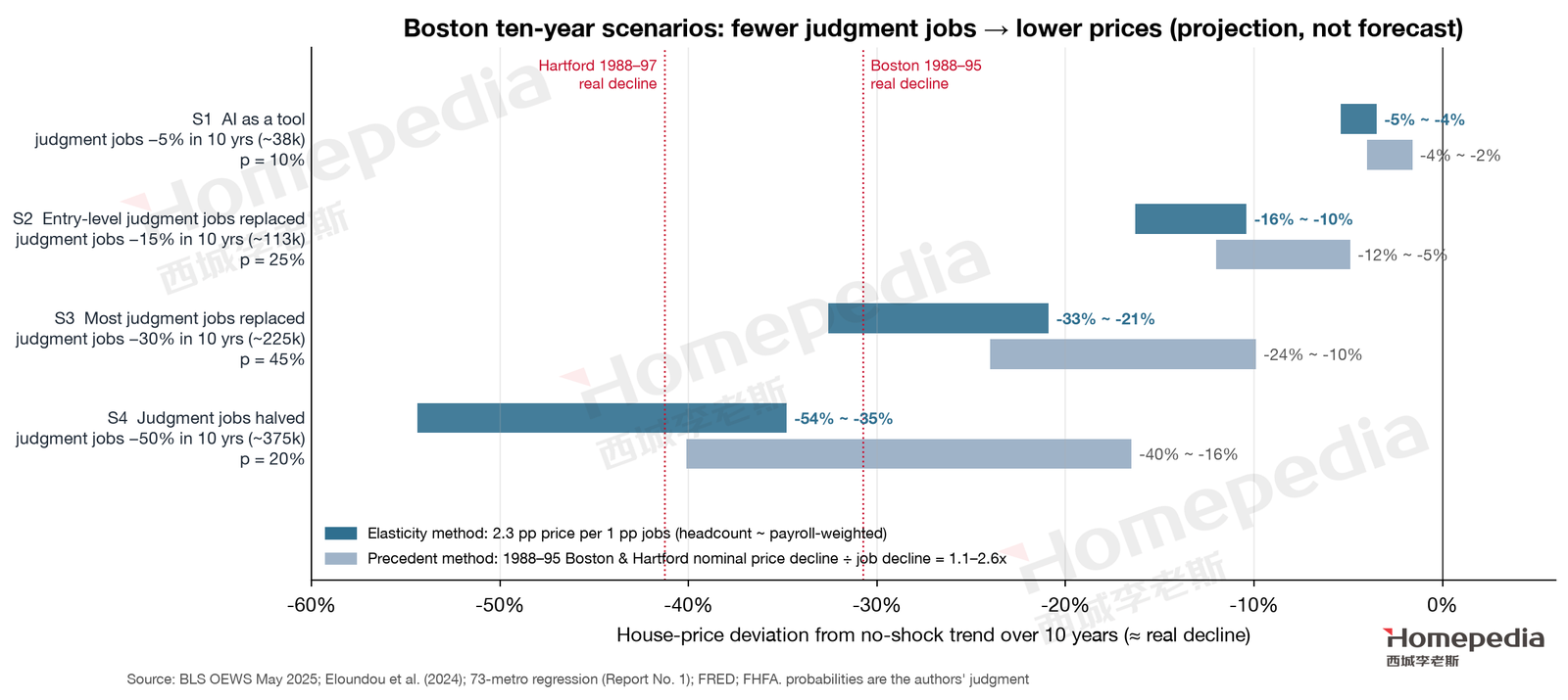
| Scenario | Net change in judgment jobs over ten years | Equivalent total employment | Elasticity method (headcount to payroll) | Precedent method (nominal) | Probability |
|---|---|---|---|---|---|
| S1 AI as a tool | −5% (about 38,000) | −1.5% | −4% to −5% | −2% to −4% | 10% |
| S2 Entry-level judgment jobs replaced | −15% (about 113,000) | −4.6% | −10% to −16% | −5% to −12% | 25% |
| S3 Most judgment jobs replaced | −30% (about 225,000) | −9.1% | −21% to −33% | −10% to −24% | 45% |
| S4 Judgment jobs halved | −50% (about 375,000) | −15.2% | −35% to −54% | −16% to −40% | 20% |
“Deviation” in the table means deviation from the no-shock trend, cumulated over ten years. If the no-shock trend is prices roughly tracking inflation (flat in real terms), the deviation approximates the real decline; the nominal decline would be smaller by an amount that depends on inflation and income growth over the decade, and income growth is itself what the shock hits. S4’s upper bound (−54%) exceeds any postwar precedent among U.S. metros (Hartford’s real decline was 41%); we read it as the edge of the model’s extrapolation rather than a plausible outcome, and put S4’s realistic range at −35% to −40%.
The scenario parameters are grounded as follows. S1 corresponds to Acemoglu’s estimate (under 5% of tasks profitably automatable). S2 corresponds to Goldman Sachs’s “7% of workers replaced” and to the path of entry-level contraction with the existing stock shrinking through retirement; far more than 15% of judgment-job holders will retire or change careers within ten years, so the scenario is reached simply by not hiring replacements. S3 corresponds to the IMF’s “half of exposed jobs face replacement” and McKinsey’s “30% of business and legal work hours,” and is the lower bound of Wei Li’s “most taken away.” S4 is an accelerated S3, in which capabilities keep improving and management jobs shrink with the number of people managed.
The probabilities are this report’s judgment, not data. We assign 65% to S3 and S4 together and 90% to S2 or worse, for three reasons. First, the institutional estimates date from 2023, and the entry-level contraction observed in 2025–2026 (a relative gap widening from 13% to 19%, six points in a year) has run faster than those estimates implied, so the distribution should shift toward more replacement. Second, Boston has the highest concentration of judgment jobs in the country, so at any given national replacement rate Boston bears a larger share. Third, ten years is long enough for “no new hiring” to replace the existing stock without waiting for layoffs. The opposing case also needs stating: S1’s 10% reflects the possibility that AI, like earlier general-purpose technologies, mainly assists, and that replaced jobs are made up by new ones. Historically that has been the norm and cannot be excluded. We give it a low probability because the group exposed this time is exactly the group that gained from every previous technological revolution, and the “new jobs make up the difference” mechanism has not yet shown evidence of working for them.
On this distribution, the probability that Boston prices fall more than 10% relative to trend within ten years is about 90%, and the probability of a fall of more than 20% (matching or exceeding the real decline of 1988–1995) is about 65%. That is our quantitative reading of “very likely to fall substantially”: a substantial fall means a real adjustment on the scale of the early 1990s, not nominal prices halving.
10.5 Offsetting Factors and Their Limits
Six factors could make the outcome better than the projection above. Each deserves an honest statement and a reply.
Health care and education are growing, and their exposure is low. This is the strongest counter-evidence: health care is Boston’s only large sector still growing (§2), and health care and education together hold 374,000 jobs with exposure of 0.35–0.38. But they are only 16.6% of payroll, and only 36,000 of their jobs pay $150,000 or more, less than an eighth of the high-paying judgment jobs. The hospital system can support ordinary owner-occupied homes and rentals in Quincy, Medford and the gateway cities; it cannot support prices in Brookline, Wellesley and Cambridge. And a considerable share of teaching-hospital and university revenue comes from research funding, which is contracting (§3), and tuition, which depends on international students, who are becoming fewer (§8).
AI will create new jobs in Boston. The clustering of AI drug discovery and AI research groups noted in §4 is real. But the number and location of the new jobs are uncertain: the industries that replaced the minicomputer in the 1990s went elsewhere [35], and Boston’s information employment is 14.8% below late 2019 with no net addition from a new industry yet. Even if AI drug discovery succeeds, its business logic is to do more research with fewer scientists, consistent with Wei Li’s observation that pharma can boom while needing fewer scientists. New jobs will come, but there is no evidence yet that they can replace hundreds of thousands of judgment jobs within ten years.
International migration will keep replenishing demand. Net international migration of about 58,000 a year in 2022–2024 was the whole of Boston’s population growth (§5). But in 2025 it already halved to 31,000, and more importantly, international migrants come to Boston for universities, hospitals, research and tech jobs; if judgment jobs contract, the inflow contracts with them. They almost all rent on arrival, and their support for the owner-occupied market shows up only years later.
Rates will fall. Rates are national; the 73-metro regression already places them in the common trend. They set the level for every city but not Boston’s deviation from other cities. Rates fell three points in 1989–1993 and Boston prices still fell 12–16%. Lower rates would make the nominal decline in every scenario somewhat smaller; they would not change the ordering of the scenarios.
Supply is minimal and owners have little leverage, so no one is forced to sell. This is why prices cannot fall within two years. Over ten years it turns around: minimal supply means prices are set entirely by demand, with no “builders stop building” buffer when demand falls (Dallas has one); low leverage means no one is forced to sell, but sales from retirement, relocation and death do not stop, and someone has to buy those homes. Owners in 1989–1992 were not forced to sell either, and prices still completed their adjustment within three years.
The wealth and existing income of high-income households. Even if the jobs disappear, accumulated wealth (equity, retirement savings, existing homes) remains. That slows the decline, and is why the adjustment takes ten years rather than two, but it does not change the direction: prices are set by the marginal buyer, and the marginal buyer over the next decade is a household that must reach the $195,000 threshold on new income.
Taken together, only one of these six factors could change the order of magnitude: the number of new jobs AI creates in Boston. The other five affect only the speed and the nominal size. That is why, on a ten-year horizon, only one indicator needs watching: whether the number of Boston jobs in occupations paying $150,000 or more (OEWS, updated each May, currently 320,000) is rising or falling.
10.6 Why Two Years and Ten Years Do Not Contradict Each Other
This report’s two judgments on Boston, that overall prices cannot fall within two years and that they are very likely to fall substantially within ten, look opposed, but they are the same mechanism seen on two time scales. Within two years, prices are set by sellers: owners holding 3% mortgages do not sell, new homes cannot be built, inventory is 80% of pre-pandemic, and a home sells in 43 days; as long as the number of buyers does not fall to zero, prices are supported. Within ten years, prices are set by buyers: some of today’s owners will have to sell, and whoever takes over must be a new household earning close to $200,000, and in Boston such households come mainly from judgment jobs. Supply constraints protect prices over two years and amplify their fall over ten. Boston in 1988–1995 followed exactly that path: employment started falling in mid-1989, prices did not bottom until 1992, and five more years passed before they regained their peak.
The right way to read the two judgments is therefore: two years, watch inventory; ten years, watch jobs. The scenarios and leading indicators of §11 address the former; the property-type outlook and strategy of §12–§13 give the implications on both horizons.
11. Scenario Analysis and Leading Indicators: The Next Two Years
This section’s three scenarios and eight leading indicators cover the next 12–24 months. The ten-year scenarios are in §10.4; the end of this section sets the two side by side and names the one indicator to track over ten years.
| Upside (~20%) | Base (~60%) | Downside (~20%) | |
|---|---|---|---|
| Overall price direction (12–24 months) | Modest gains of 3–6% | Gains of 0–3%, low volume | Flat to −3–5%, volume falls sharply |
| Conditions | Research funding restored and life-sciences financing recovers; rates below 6% | Health care jobs grow steadily; no further sharp cuts to research funding; rates 6.5–7.5% | Research funding and white-collar jobs keep contracting; rates above 7.5% |
| Suburban and gateway-city single-family | Lead gains | Stable to slightly higher | Mild correction |
| Core owner-occupied (incl. condos) | Catch-up gains | Keep underperforming | Lead declines |
| Core rentals | Rents accelerate | Modest rent growth | Flat rents, rising vacancy in student areas |
Base case: resilient divergence (~60%). This is the most likely path. Supply barely grows and inventory is still below pre-pandemic, so overall prices are hard to push down; but buying requires 1.66 times median income and rates are back above 7%, so buyers are few and volume stays low. Stable hospital employment and the large stock of high earners are enough to support continued modest gains for single-family homes in suburban school districts and gateway cities; owner-occupied product in the core, especially condos, keeps underperforming; core rental demand stays firm.
Upside: modestly firm (~20%). The trigger is a simultaneous recovery in research and life sciences and a drop in rates. Massachusetts biopharma VC rose 25% in the first half of 2026 with several IPOs; if that recovery carries through to hiring while rates return below 6%, Boston’s “price amplifier” kicks in: by §6’s estimate, each point of job recovery could lift prices by more than 2 points. Core owner-occupied product would catch up.
Downside: volume-led slowdown (~20%). The trigger is a further contraction in federal research funding and wider life-sciences layoffs, while white-collar employment keeps weakening under AI. The amplifier then works in reverse: high-ticket outer-suburb luxury homes and core condos come under pressure first, overall prices are flat or slightly lower, and volume shrinks sharply. With extremely constrained supply and generally low owner leverage, we do not expect a steep decline within two years; a steep decline is a ten-year question, and it requires buyers to disappear rather than sellers to multiply.
The most important signal for moving between scenarios is whether research and life-sciences hiring recovers. Capital-market rebounds (VC, IPOs) typically lead hiring by 6–12 months, and hiring in turn leads core housing demand. If in late 2026 through 2027 NIH funding stabilizes, lab vacancy starts falling and professional, scientific and technical employment turns positive, Boston is moving from the base case toward the upside; if instead these indicators keep deteriorating while white-collar jobs shrink under AI, watch for the downside.
Eight leading indicators readers can track each quarter (upside / downside thresholds in parentheses):
- NIH funding to Massachusetts (NIH RePORTER): back above $3.9 billion upside; below $3.5 billion downside. FY2026: $3.67 billion.
- Lab vacancy (brokerage quarterly reports): below 15% upside; above 25% downside. Q2 2026: 21.2%.
- Massachusetts nonfarm job growth, year over year (BLS CES): >1% upside; <−1% downside. August 2026: −0.1%.
- 30-year fixed mortgage rate (Freddie Mac): <6% upside; >7.5% downside. October 1, 2026: 7.28%.
- Active inventory relative to pre-pandemic (Realtor.com): rising above 1.0× signals a shift toward balance. Currently ~0.80×, up 16% year over year.
- Median days on market (Realtor.com): above 55 days signals clearly weaker demand. September 2026: 43 days.
- Multifamily vacancy (brokerage quarterly reports): below 5% rents accelerate; above 8% rents under pressure. Q1 2026: 6.9%.
- International student enrollment (each school’s fall data): further declines would weaken rental demand in student areas.
Two years against ten. Setting this section beside §10:
| Next two years (this section) | Next ten years (§10) | |
|---|---|---|
| Who sets prices | Sellers: rate lock-in, low leverage, no new homes | Buyers: who has $200,000 of income to take over |
| Most likely path | Modest gains of 0–3%, low volume (~60%) | Judgment jobs down 30%, prices 21–33% below trend (~45%) |
| Worse path | Flat to −3–5% (~20%) | Judgment jobs halved, deviation of −35% or more (~20%) |
| Better path | Gains of 3–6% (~20%) | AI as a tool, deviation within −5% (~10%); entry-level jobs replaced, −10% to −16% (~25%) |
| Main source of risk | Research funding, life-sciences financing, rates | AI replacing management, finance, computing, research and legal jobs |
| Indicators to track | The eight above | One: Boston jobs in occupations paying $150,000 or more (OEWS; currently 320,000) |
There is only one ten-year indicator because, as §10 showed, the other factors (rates, migration, health care growth, scarce supply) change only the speed and the nominal size, not the direction; only the number of high-paying jobs can change the direction. OEWS publishes the prior year’s data each May, so readers need check once a year. If the number falls for two consecutive years, the ten-year judgment is coming true; if it keeps rising, the new jobs AI creates are landing in Boston and the ten-year judgment needs revising.
12. Outlook by Property Type
| Property type | Map view | Two-year conclusion | Key evidence | Ten-year view (§10) |
|---|---|---|---|---|
| Luxury single-family | Neutral | Suburban school districts firm; core luxury soft | Wellesley +15.0% and Newton +11.0% over three years; Brookline −4.3% | First in line: buyers come almost entirely from high-paying judgment jobs |
| Primary homes | Stable | Stable, led by gateway cities | Bottom tier +56.4% since 2019; Lowell and Brockton +10%+ over three years | Relatively the steadiest: health care and education jobs can support this segment |
| Condos | Split | Underperforming; depends on building and transit | +31.3% since 2019 vs. +47.4% overall; core towns lag | Soft: core buyers are precisely the most exposed group |
| Rental homes | Firm | Firm, especially in the core | Core rents rose about twice as fast as values; 39% of households rent | Cash flow steady, appreciation not to be counted on: entry-level white-collar tenants are hit first |
| Student housing | Firm | Firm long-term; short-term pressure from international students | ~152,000 college students in the city; fewer international grad students in 2025 | Depends on the school: top schools steady, schools reliant on international graduate students riskier |
| Multifamily | Selectively firm | Selectively firm | 68% of new permits are multifamily, but totals are tiny; 6.9% vacancy | Value on rent, not appreciation |
The “two-year conclusion” column follows the evidence of the preceding sections; the “ten-year view” comes from §10. If high-paying judgment jobs fall sharply within ten years, the hardest-hit property types are those that depend on that buyer pool (core luxury, top-school-district single-family, core condos), and the least affected are the ordinary owner-occupied homes and rentals supported by health care, education and middle-income households in the gateway cities.
Luxury single-family. The map calls this segment “neutral: scarce, yet sensitive to bonus and equity income.” Over two years that holds; over ten, this is the segment most sensitive to §10’s conclusion, since 89% of the 320,000 jobs paying $150,000 or more are judgment jobs, and that is precisely the buyer pool for top suburban school districts and core luxury. The data show sharp internal divergence: suburban school districts (Wellesley, Newton, Lexington) rose 10–15% over three years, while core luxury (Brookline) fell 4.3%. Suburban luxury buyers are physicians, lawyers and senior executives with stable incomes; core luxury buyers come more from life sciences and tech, with incomes tied to equity and bonuses—the groups hit hardest since 2023.
Primary homes ($500,000–$800,000). This is Boston’s steadiest segment. Gateway cities and outer towns (Lowell, Brockton, Lynn, Salem, Framingham) rose 46–59% since 2019 and still 9–12% over the past three years. They serve middle-income households priced out of the core and have commuter rail into the city. New multifamily from the MBTA Communities Act has limited effect here because the volume is so small.
Condos. Boston condos are up only 31.3% since 2019, well behind the overall market (47.4%). Condo buyers must evaluate the building: newer buildings near transit and job centers with healthy reserves and no recent special assessments clearly outperform older ones. Older buildings face facade, roof, elevator and energy-retrofit costs.
Rental homes. Over two years, one of the categories we favor most, especially in the core. The monthly cost gap between owning and renting exceeds $1,100, keeping many would-be buyers in the rental market. But investors need to do the math, and to take ten-year appreciation out of it:
Example: the return on a typical single-family rental
Purchase price $733,574, rent $3,648 a month, annual rent $43,776: a gross yield of about 6.0%. Subtract property tax (at 1.3%) of about $9,540, insurance of about $3,000, and vacancy, repairs and management (20% of rent) of about $8,760, and net operating income is about $22,480—a cap rate of about 3.1%, below the 7.28% mortgage rate. As in Dallas, Boston rentals at today’s rates suit all-cash or low-leverage ownership, and the return can only come from rent. Investors used to say “the cash flow doesn’t work, but the long-run appreciation does.” Within §10’s framework that reasoning no longer holds: the tenants and buyers of ten years from now are exactly the people AI is most likely to replace. Measured at a 3.1% cap rate with no expectation of appreciation, a Boston rental at today’s price and rate is not a good investment.
Student housing. Boston has the densest university cluster in the country, so student housing demand is structural; most universities’ on-campus housing falls far short of demand, and many upper-class undergraduates and almost all graduate students rent off campus. In the short run, fewer international graduate students in 2025 raised vacancies around Northeastern and Mission Hill. Investors should check each school’s dependence on international graduate students: top schools such as Harvard and MIT are largely unaffected, while schools that rely on international graduate enrollment carry more risk.
Multifamily. 68% of Boston’s new permits are multifamily, but the total is too small for new supply to push rents down. Vacancy rose from low levels to 6.9%, mainly due to fewer students and concentrated deliveries. Near the core and major transit, new multifamily remains well supported; in areas far from transit and reliant on students, caution is warranted. The MBTA Communities Act will add multifamily along commuter rail lines over the medium to long term—mild competition for existing assets, but at its current scale of about 7,000 homes it won’t change the tight core rental market for several years.
13. Strategic Implications for Market Participants
13.1 Buyers
- First ask how many years you plan to stay. This is where the two-year and ten-year judgments meet. If you are buying to live in and plan to stay five years or less, Boston is a safe market: prices will not fall within two years, and the decision can be made normally by the points below. If you plan to stay ten years or more, or if “Boston will certainly be worth more in ten years” is part of your reason for buying, §10’s projection says that reason most likely does not hold. Buy on the basis of what you can afford and what the home is worth to live in, not on appreciation, and leave room in the budget for prices to fall 20–30% without disrupting your life.
- Accept the reality of little negotiating room and a slow pace. Boston homes sell faster than before the pandemic and only 16.6% of listings have cut prices. Good homes still draw multiple offers; expecting deep discounts is unrealistic.
- Prioritize gateway cities and the inner ring. Towns such as Lowell, Quincy and Malden, with commuter rail or subway access, have typical prices 30–50% below Cambridge and Brookline, and have seen larger gains and steadier demand in recent years.
- Do your homework on condos. Ask for the building’s budget, reserve study, recent special assessments and insurance renewal history; budget for future major repairs in older buildings.
- Buy in the core only with a long horizon. Core home values have become relatively “cheap” against rents (values rose only half as fast as rents). If you plan to live there long term and value the commute and city life, now is a more reasonable entry point than in recent years—but don’t count on short-term appreciation.
- School districts are the most important variable for Chinese-American families, but separate the “school premium” from the “commute premium.” Newton, Lexington, Wellesley and Brookline have long been known for strong public schools, and suburban school-district towns have clearly outperformed the core over three years, showing the school premium remains strong; yet Brookline, also a renowned district, fell 4.3% over three years, showing that changes in the core’s product and buyer mix can offset a school advantage. When choosing a town, look at Massachusetts Department of Elementary and Secondary Education (DESE) school data, the commute to work, and the town’s recent new construction and zoning changes.
- Count the full carrying cost. Massachusetts property tax rates are lower than Texas’s, but prices are high, so the dollar amount is not small. Owner-occupants in Boston can apply for the residential exemption, which can lower the tax bill substantially.
13.2 Sellers
- If you were going to sell anyway, these two years are the window. Over the next two years prices are at a high, sales are slow but prices do not fall; over ten years prices are very likely to move clearly lower. Owners whose children have grown and who want to change cities, who are retiring and moving away, or who hold core luxury homes and condos have no reason to wait: waiting will not bring a higher price within two years, and within ten it will bring a lower one.
- Suburban and gateway-city sellers are in a strong position. Inventory is low and homes sell quickly; sensible pricing is enough.
- Core condo sellers need more competitive pricing. Core condos lag the market and buyers have more choice; price against recent sales in the same building, not 2022 highs.
- Use the spring window. Boston’s market is strongly seasonal; buyer numbers and prices in spring (March–June) are clearly higher than in fall and winter. If time allows, list in spring and complete repairs and preparation over the winter.
- Core sellers can consider renting first, but set a deadline. If you don’t need to cash out, rental demand in the core is firm, and you can wait for a research and life-sciences recovery before selling. But limit the wait to two years; if after that the number of jobs paying $150,000 or more is still falling, do not push the sale out toward the ten-year horizon.
13.3 Investors
- Do not buy Boston for long-run appreciation. This is the ten-year judgment’s most direct implication for investors. At a 3.1% cap rate against a 7.28% mortgage rate the cash flow does not work, and the “long-run appreciation” that used to make up for it does not hold within §10’s framework. Anyone who still wants to hold Boston assets should value them on rent alone, use all cash or low leverage, and check the number of jobs paying $150,000 or more once a year.
- Core rentals are Boston’s best rental assets over two years, but accept net yields of about 3% and returns that rely on rent rather than appreciation.
- For student housing, look at the school, not the market. Avoid areas overly dependent on international graduate students.
- Primary homes in gateway cities are a steady long-term choice. Lowell, Lynn and Brockton offer relatively low prices, commuter rail access and stable rental demand, with both prices and rents rising in recent years; zoning relaxation under the MBTA Communities Act may also create opportunities for small-scale multifamily conversions.
- Over two years watch research funding and lab vacancy; over ten watch the count of high-paying jobs. The first two are leading signals of demand over two years, and once a clear recovery appears, core owner-occupied product may catch up; the third is the only indicator of whether the ten-year judgment is coming true.
- A note for Chinese investors. Real estate transactions in Boston and Massachusetts are attorney-led, and condo purchases involve extensive document review; before investing across state lines, retain a local attorney and an agent familiar with local zoning.
14. Limitations and Risks
- Research funding is highly policy-dependent. Our base case assumes no further sharp cuts to federal research funding. A new round of cuts—or, conversely, a large restoration—could move Boston’s demand and prices away from the base case.
- The price amplifier works both ways, and the 2.3 multiple was estimated from short-run data. §6’s regression uses a 2019–2026 cross-section of 73 metros and captures the price response over six or seven years. Extrapolating it to ten years introduces error in both directions: over a decade supply can respond to a limited degree (though Boston adds only about 10,000 homes a year, so the response is small), which would make the multiple smaller; and the knock-on contraction of local services and the out-migration that follow the loss of high-paying jobs are not counted, which would make it larger. The 1988–1995 precedent (multiples of 1.1–2.6 nominal and 2.7–5 real) provides an external check, but the precedent itself contains a bubble-bursting component.
- §10’s ten-year scenarios are projections, not forecasts. No data can establish the replacement rate for judgment jobs; we can only set scenarios from institutional estimates (4.6% to 30%) and two years of early observation. The scenario probabilities are this report’s subjective judgment, and readers may substitute their own. The decade may bring outcomes we have not imagined: AI creating enough new jobs in Boston, major policy intervention, or AI capabilities advancing more slowly than in the past two years. The ten-year judgment should be revised as each year’s OEWS data arrive.
- AI exposure measures technical potential. The exposure scores were built in 2023, and model capabilities have advanced markedly since, so the scores may understate exposure in management and similar occupations; conversely, exposure does not guarantee replacement, and actual effects depend on how firms use AI and whether new jobs appear.
- The core’s shift may be structural. Remote and hybrid work mean some white-collar workers no longer need to live near downtown; if this persists, the core’s lag in owner-occupied demand may not fully reverse with an economic recovery.
- Data limitations. Zillow’s town and ZIP data are smoothed; town-level rent samples are small; QCEW and CES use slightly different geographies for Boston (CES covers only the Massachusetts portion); FY2026 NIH data run through early October and may be revised slightly; the 1988–1995 employment series are state-level because metro monthly series begin only in 1990; OEWS “payroll” is employment times mean annual pay by occupation and is an approximation.
Even so, we believe both of the report’s core arguments rest on basic facts. The two-year argument—extremely constrained supply converts the knowledge economy’s resilience into stable home prices, while affordability constraints make core rentals better supported than ownership—follows from geography, institutions and income structure, and will not change within two years. The ten-year argument—supply constraints can hold up prices but cannot create buyers; Boston’s buyers are concentrated in high-paying judgment jobs, which are exactly the work AI is most likely to replace within a decade; and supply that scarce will then amplify the contraction in demand into a fall in prices—is the same set of facts carried over a longer horizon. Prices that cannot fall in two years and prices very likely to fall substantially in ten are two faces of the same market on two time scales: two years, watch inventory; ten years, watch jobs.
Appendix A: Methodology and Data Sources
Employment and wages. Metro employment comes from BLS QCEW annual averages for 2019 and 2024 (all ownerships); industry analysis uses private-sector NAICS supersectors. Monthly trends use BLS CES data for the Massachusetts portion of the Boston-Cambridge-Newton metro; total employment is seasonally adjusted and industry series are 12-month moving averages of non-seasonally-adjusted data.
Research funding. NIH awards come from the NIH RePORTER API (organization state = Massachusetts), summed by fiscal year; FY2026 data run through early October 2026. Lab vacancy comes from Lincoln Property Company’s Q2 2026 report; biopharma employment from MassBio’s 2026 Industry Snapshot.
AI exposure. BLS OEWS May 2025 occupational data matched to the β exposure scores of Eloundou et al. (2024), covering 93.3% of Boston employment; “highly exposed” means β ≥ 0.5. §10’s “judgment occupational groups” are SOC 11, 13, 15, 17, 19 and 23; “payroll” is the sum of employment × mean annual pay by occupation (restricted to occupations matched to an exposure score and with wage data); pay bands are by occupational mean annual pay.
1988–1995 precedent. Massachusetts and Connecticut nonfarm employment (FRED: MANAN, CTNAN, not seasonally adjusted, 12-month moving average); S&P CoreLogic Case-Shiller Boston index (FRED: BOXRSA, seasonally adjusted); FHFA all-transactions index (Boston division, Hartford metro); CPI-U (FRED: CPIAUCSL) for inflation adjustment; 30-year fixed mortgage rate (FRED: MORTGAGE30US). Peaks and troughs are defined on each series itself; “regained peak” is the first return to the peak level.
Ten-year scenarios. The elasticity method uses Boston’s slope of 2.28 from §6’s regression; the precedent method uses the 1988–1995 ratio of price decline to job decline in Boston (FHFA nominal) and Hartford (1.1–2.6). The basis for scenario parameters and probabilities is in §10.4.
Population and migration. Population and components come from Census Vintage 2025 metro estimates. Migration income comes from IRS county-to-county migration data (tax years 2019–20 through 2022–23); “other states” means U.S. states other than Massachusetts and New Hampshire; average AGI = total AGI ÷ returns.
Housing supply. Building permits come from Census BPS county annual data for seven counties (Suffolk, Middlesex, Norfolk, Essex and Plymouth, plus Rockingham and Strafford in New Hampshire). Supply elasticity comes from Saiz (2010). The cross-metro regression is described in Report No. 1’s appendix (73 metros; interaction −2.43, p < 0.001).
Prices, rents and inventory. Prices use Zillow ZHVI (metro, ZIP and town; the ZIP analysis covers 271 ZIP codes); rents use Zillow ZORI (metro and town); inventory, price cuts, new listings and days on market come from Realtor.com. Affordability uses Zillow’s new-homeowner income needed (20% down); median income comes from ACS 2024 one-year estimates.
Reproducibility. All download scripts, charting code, raw data and intermediate statistics are archived in the project’s scripts/ (city_figures.py; cities/fig_boston_10yr.py for §10) and shared_data/ directories; the number check for §10 is in review/stage_10yr_check.md.
Data cutoffs. QCEW 2024; CES August 2026; OEWS May 2025; population estimates July 2025; IRS migration 2022–23; FHFA 2026Q2; Zillow August 2026; Realtor.com September 2026; NIH early October 2026; mortgage rate October 1, 2026; FRED historical series downloaded October 19, 2026.
References
[1] U.S. Bureau of Labor Statistics. Quarterly Census of Employment and Wages, annual averages 2019 and 2024. https://www.bls.gov/cew/ [2] U.S. Bureau of Labor Statistics. Current Employment Statistics (State and Metro Area), Boston-Cambridge-Newton, MA (Massachusetts portion), through August 2026. https://www.bls.gov/sae/ [3] U.S. Bureau of Labor Statistics. Occupational Employment and Wage Statistics, May 2025. https://www.bls.gov/oes/ [4] Massachusetts Biotechnology Council (MassBio). (2026). 2026 Industry Snapshot. https://www.massbio.org/industry-reports/industry-snapshot/ ; WBUR (2026, August 25). Mass. biopharma industry loses jobs, but investment rebounds. [5] National Institutes of Health. NIH RePORTER (API v2), projects with organization state = MA, fiscal years 2019–2026. https://reporter.nih.gov/ [6] GBH News. (2025, June 16). Massachusetts scientists have lost billions in federal funds. Now they have their day in court. https://www.wgbh.org/news/local/2025-06-16/massachusetts-scientists-have-lost-billions-in-federal-funds-now-they-have-their-day-in-court [7] Lincoln Property Company. (2026). Lab Market Report: Boston, Cambridge, Suburbs, Q2 2026. https://lpc.com/wp-content/uploads/LabMarketReport_Boston_Q2_2026_v3.pdf [8] Eloundou, T., Manning, S., Mishkin, P., & Rock, D. (2024). GPTs are GPTs: Labor market impact potential of LLMs. Science, 384(6702), 1306–1308. [9] Dodini, S., & Smith, T. (2026, September 1). Job postings show early signs of AI automation impact. Dallas Fed Economics. https://www.dallasfed.org/research/economics/2026/0901 [10] Brynjolfsson, E., Chandar, B., & Chen, R. (2026, August; first version August 2025). Canaries in the Coal Mine? Six Facts about the Recent Employment Effects of Artificial Intelligence. Stanford Digital Economy Lab. https://digitaleconomy.stanford.edu/app/uploads/2026/08/Canaries_August2026.pdf [11] U.S. Census Bureau. Metropolitan Population Totals and Components of Change, Vintage 2025 and Vintage 2020. https://www.census.gov/programs-surveys/popest.html [12] Internal Revenue Service, Statistics of Income. County-to-County Migration Data, 2019–2020 through 2022–2023 (inflow and outflow files). https://www.irs.gov/statistics/soi-tax-stats-migration-data [13] Zillow Research. ZHVI (metro, ZIP, city), ZORI (metro, city), and affordability series, through August 2026. https://www.zillow.com/research/data/ [14] U.S. Census Bureau. American Community Survey 2024 1-Year Estimates, Tables B19013, B25003, B25064, B25070, B25077 (via Census Reporter). https://censusreporter.org [15] Freddie Mac. Primary Mortgage Market Survey, week of October 1, 2026. https://www.freddiemac.com/pmms [16] City of Boston. FY26 tax rates (residential $12.40 and commercial $26.96 per $1,000). https://www.boston.gov/departments/assessing/how-we-tax-your-property [17] Realtor.com Economic Research. Residential Data, Metro Core Metrics, through September 2026. https://www.realtor.com/research/data/ [18] Glaeser, E. L., & Ward, B. A. (2009). The causes and consequences of land use regulation: Evidence from Greater Boston. Journal of Urban Economics, 65(3), 265–278. [19] The Boston Foundation. (2026, January). Review of early results of MBTA Communities Act finds law has produced “real but modest” gains. https://www.tbf.org/news-and-insights/press-releases/2026/january/mbta-communities-report-pr-202601 ; Boston.com (2026, January 27). MBTA Communities Act: What’s next for your town. [20] U.S. Census Bureau. Building Permits Survey, county annual files 2015–2025. https://www.census.gov/construction/bps/ [21] Saiz, A. (2010). The geographic determinants of housing supply. Quarterly Journal of Economics, 125(3), 1253–1296. [22] Federal Housing Finance Agency. House Price Index, All-Transactions, metropolitan statistical areas and divisions, through 2026Q2. https://www.fhfa.gov/data/hpi [23] The Boston Globe (2025, September 15). An uptick of apartment vacancies in Boston suggests a decline in student enrollment; WBUR (2025, November 10); GBH News (2025, November 17). International student enrollment falls sharply in US, early data show. https://www.wgbh.org/news/education-news/2025-11-17/international-student-enrollment-falls-sharply-in-us-early-data-show [24] Boston Planning & Development Agency. Boston by the Numbers: Colleges and Universities. https://www.bostonplans.org/getattachment/1770c181-7878-47ab-892f-84baca828bf3 [25] Colliers. (2026). Greater Boston Multifamily Report, 2026 Q1. https://www.colliers.com/en/research/boston/greater-boston-multifamily-report-2026q1 [26] Matthews Real Estate Investment Services. (2026). Boston, MA Multifamily Market Report, August 2026. https://www.matthews.com/insights/boston-multifamily-august-2026 [27] GBH News (2026, June 23). Rent control question disqualified due to religious exemption; Greenberg Traurig (2026, June). Massachusetts high court takes rent-control initiative off 2026 ballot. https://www.wgbh.org/news/politics/2026-06-23/rent-control-question-disqualified-due-to-religious-exemption [28] Briggs, J., & Kodnani, D. (2023, March 26). The Potentially Large Effects of Artificial Intelligence on Economic Growth. Goldman Sachs Global Economics Analyst; summary: Goldman Sachs (2023, April 5). Generative AI could raise global GDP by 7%. https://www.goldmansachs.com/insights/articles/generative-ai-could-raise-global-gdp-by-7-percent [29] Cazzaniga, M., Jaumotte, F., Li, L., Melina, G., Panton, A. J., Pizzinelli, C., Rockall, E., & Tavares, M. M. (2024). Gen-AI: Artificial Intelligence and the Future of Work. IMF Staff Discussion Note SDN/2024/001. https://www.imf.org/en/publications/staff-discussion-notes/issues/2024/01/14/gen-ai-artificial-intelligence-and-the-future-of-work-542379 [30] McKinsey Global Institute. (2023, July 26). Generative AI and the future of work in America. https://www.mckinsey.com/mgi/our-research/generative-ai-and-the-future-of-work-in-america [31] Acemoglu, D. (2025). The simple macroeconomics of AI. Economic Policy, 40(121), 13–58 (NBER Working Paper 32487, 2024). https://www.nber.org/papers/w32487 [32] World Economic Forum. (2025, January). The Future of Jobs Report 2025. https://www.weforum.org/publications/the-future-of-jobs-report-2025/ [33] Case, K. E. (2000). Real estate and the macroeconomy. Brookings Papers on Economic Activity, 2000(2), 119–162. https://www.brookings.edu/wp-content/uploads/2000/06/2000b_bpea_case.pdf [34] Federal Reserve Bank of St. Louis, FRED. Series MANAN and CTNAN (BLS state nonfarm employment, not seasonally adjusted), BOXRSA (S&P CoreLogic Case-Shiller MA-Boston Home Price Index, seasonally adjusted), CPIAUCSL, MORTGAGE30US (Freddie Mac PMMS). Downloaded October 19, 2026. https://fred.stlouisfed.org/ [35] Saxenian, A. (1994). Regional Advantage: Culture and Competition in Silicon Valley and Route 128. Harvard University Press. [36] Moretti, E. (2010). Local multipliers. American Economic Review, 100(2), 373–377.
Disclaimer: This report is for research and educational purposes only and does not constitute investment, legal or tax advice. Real estate investing involves risk; readers should consider their own circumstances and consult licensed professionals.