

Data as of writing This report was completed in October 2026 using the latest public data available at the time; sources are cited in the text and references. Markets keep moving, so some figures may have changed by the time you read this. The framework and the way of reading the market still hold; check current data for the latest figures.
© 2026 Wei Li · Homepedia. All rights reserved. The text, data and charts in this report are protected by copyright and may not be copied, republished, excerpted or used commercially without written permission.
Abstract
San Diego is the market in this three-city series where prices have risen the most and housing is least affordable. From December 2019 to August 2026, San Diego’s typical home value rose 54.4% to $930,785, more than Boston (47.4%), the U.S. (47.9%) and Dallas (37.5%). The typical home costs 8.5 times median household income, and buying one requires household income of about $237,000, 2.17 times the median. Over the same period, San Diego’s employment grew only 3.2%, and the metro lost 17,000 to 41,000 residents a year to net domestic out-migration.
This report asks why a metro with limited demand growth and extremely poor affordability posted the largest price gains, and how durable those gains are. Our central thesis—the one Wei Li stated on the SeaHomepedia Housing Map—is: defense, biotechnology and R&D investment give San Diego a base of high-income employment, and topography and land scarcity tightly restrict supply, so prices stay firm over the long run; but extremely low affordability makes this market unusually sensitive to any change in its affluent buyers.
We test the thesis with 20 charts built from public data. Supply: Saiz (2010) estimates San Diego’s housing supply elasticity at just 0.67, the 5th lowest of 95 large metros; prices have risen 324% since 2000, the most of the three metros. A 73-metro regression shows that in a market like San Diego, each percentage point of job growth corresponds to about 2.9 points of price growth. Demand: defense spending accounts for 22.2% of the regional economy and supports about 357,000 jobs, a very stable foundation; but with defense contract dollars edging down, NIH funding 13% below 2024 and life-sciences lab vacancy at 28.1%, it currently acts more as a stabilizer than a growth engine; the real source of new jobs is health care. Price structure: San Diego’s divergence runs opposite to Dallas’s—over three years the priciest fifth of ZIP codes rose 11.3% while the cheapest rose only 3.0%; since 2019, high-end coastal communities are up 60–76%. This “high end leads” pattern shows that prices are supported mainly by the wealth of high-income households rather than income growth of ordinary families—which is precisely the source of fragility.
Our base case is “slow and firm”: over the next 12–24 months, scarce supply continues to hold up prices and overall values rise modestly, but high payments keep volume and liquidity low; high-end coastal communities are strongest but most volatile, entry-level product and condos are weak, and rental demand stays firm. The main risk lies in affluent buyers’ wealth and income—equities, biotech financing and the defense budget. If they weaken together, high-end product will adjust first.
Key Findings
- Largest gains, worst affordability of the three: up 54.4% since 2019; homes cost 8.5 times income, and buying requires 2.17 times median income.
- Supply tightly constrained by topography: Saiz elasticity 0.67, the 5th hardest place in the U.S. to build; permits per resident are less than half of Dallas’s.
- Defense stabilizes, health care adds jobs: defense is 22.2% of the regional economy, but contract dollars are edging down; job gains come mainly from health care (+34% since 2019).
- The high end leads, the low end stalls: the priciest fifth of ZIPs is up 75% since 2019, the cheapest 41%; over three years, 11.3% vs. 3.0%.
- The market is slowing: homes sit about 10 days longer than before the pandemic, price cuts are rising and condos are 7% below peak; new listings are only 65% of pre-pandemic as rate lock-in depresses sales.
- The strongest rental demand of the three: 45.6% of households rent, 58% of renter households pay over 30% of income in rent, and rents are up 44% since 2019.
- Insurance is a new carrying-cost risk: California FAIR Plan policies in San Diego County rose 57.8% in a year, and insurance costs in hillside and high-wildfire-risk areas have risen sharply.
1. Introduction: Research Questions and Central Thesis
The single most important sentence about San Diego is this: supply here can barely respond, so the direction of prices depends almost entirely on the condition of affluent buyers.
San Diego is bounded by the Pacific to the west, the Mexican border to the south, mountains and desert to the east and Marine Corps Base Camp Pendleton to the north, and its urban area is cut by numerous canyons and preserves. Developable flat land was used up long ago; what remains is too steep, in high wildfire-risk zones, or tightly restricted by the Coastal Commission and environmental review. An estimated supply elasticity of just 0.67 means nearly every increment of demand turns into price.
In such a market, prices are set by those who can pay. San Diego’s high-income jobs come from defense, biotechnology, communications technology (such as Qualcomm) and top research institutions (UC San Diego, Scripps Research, the Salk Institute), plus many retirees and remote workers who arrive with wealth. As long as their incomes and wealth grow, they bid up the limited housing stock; when their circumstances change, prices—especially at the high end—are hit first. That is what Wei Li means by “firm but fragile.”
Compared with California’s other big metros, the San Francisco Bay Area and Los Angeles, San Diego’s economy is steadier: the Bay Area depends heavily on tech, with prices rising and falling with tech stocks and hiring; Los Angeles relies on entertainment, trade and a broader service economy. San Diego has two cornerstones largely immune to the business cycle—defense and health care—plus high-pay jobs in biotech and communications technology. So its prices usually swing less than the Bay Area’s, but affordability is just as extreme. This combination of “a stable base but fragile buyers” is the core of this report.
The SeaHomepedia Housing Map scores San Diego on five dimensions; this report provides the evidence for each:
| Dimension | Map rating | Evidence in this report (section) | Verdict |
|---|---|---|---|
| AI job risk | Med–low | 29.8% of jobs highly exposed, the lowest of the three metros (§5) | ✓ Supported |
| Infrastructure upside | High | Defense is 22.2% of the regional economy; naval and defense-industrial infrastructure is a long-run foundation, though contract and research dollars have recently declined (§3–4) | ✓ Partly supported |
| Marginal affluent buyer | Modestly rising | High-end leadership shows strong affluent demand, but it comes mainly from existing wealth; arrivals do not earn more than departures (§6, §8) | ✓ Partly supported |
| Supply elasticity | Low | Saiz elasticity 0.67, 5th lowest in the U.S.; permits per resident less than half of Dallas’s (§7) | ✓ Strongly supported |
| Price pressure | Firm but fragile | Largest gains of the three and still near peak, but longer days on market, more price cuts and condos retreating (§8) | ✓ Strongly supported |
2. Economic Fundamentals: The Triangle of Defense, Health Care and Research
2.1 Employment Growth
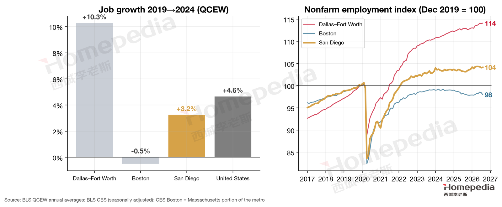
According to the BLS QCEW, average employment in the San Diego metro grew from 1.488 million in 2019 to 1.537 million in 2024, up 3.2% over five years—below the U.S. (4.6%) and far below Dallas (10.3%), but better than Boston (−0.5%) [1]. Monthly data show nonfarm employment of 1.575 million (seasonally adjusted) in August 2026, 4.1% above December 2019 and up about 1% over the year [2].
San Diego had the fastest wage growth of the three: average annual pay across all industries rose from $64,211 in 2019 to $82,854 in 2024, up 29.0%, above the national 27.7% [1]. In level, however, San Diego’s average pay is close to the national average and well below Boston’s ($103,714), while its home prices are the highest of the three. This combination of “average income, highest prices” is the direct cause of extreme unaffordability.
2.2 Industry Composition
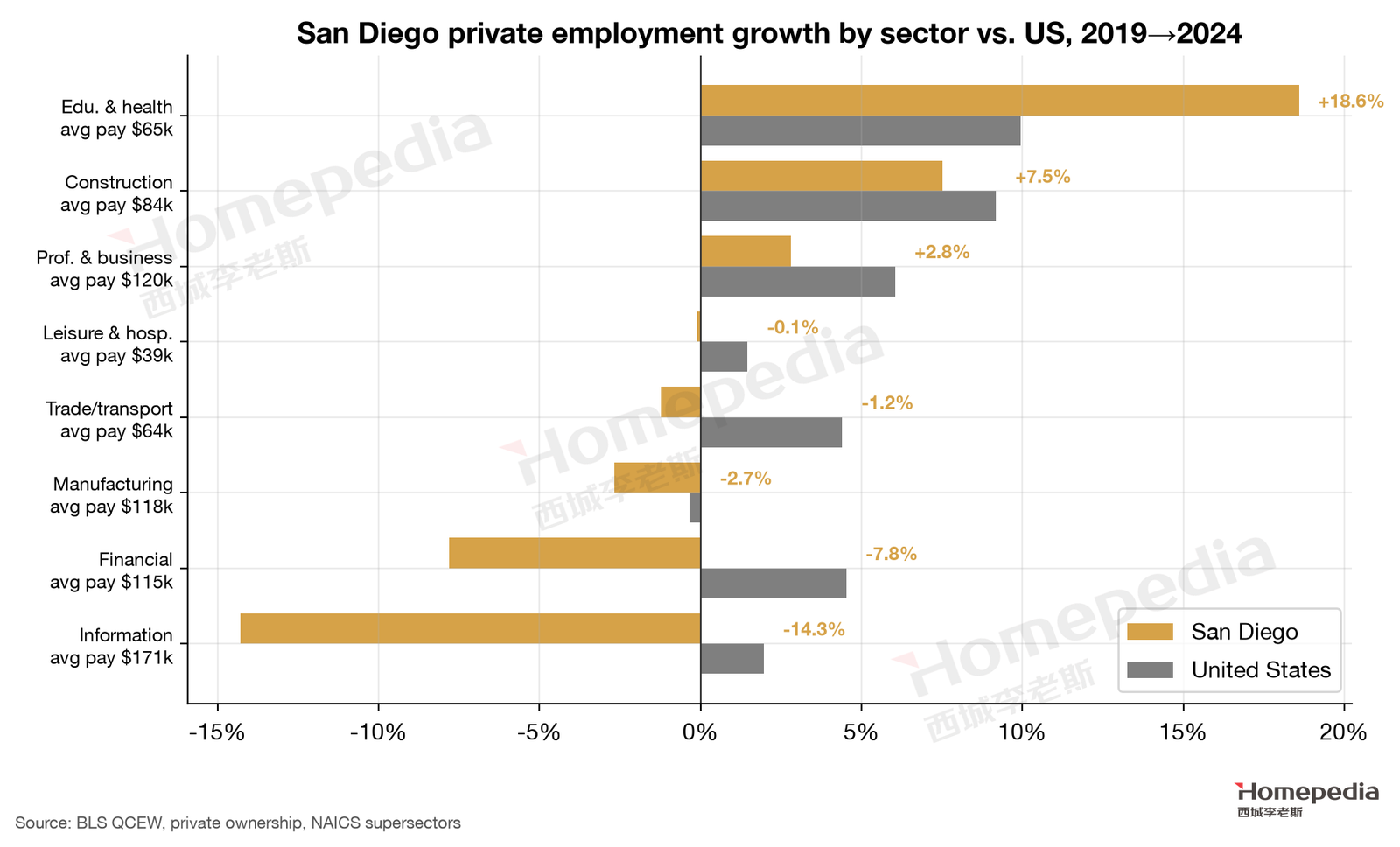
By sector (Figure 2), the fastest-growing industry in San Diego from 2019 to 2024 was education and health (+18.6%, about 250,000 jobs, vs. +10.0% nationally), followed by construction (+7.5%) and professional and business services (+2.8%, about 261,000 jobs, average pay $119,589). Shrinking industries included information (−14.3%, average pay $171,028), finance (−7.8%), manufacturing (−2.7%, average pay $118,398) and trade/transportation (−1.2%) [1].
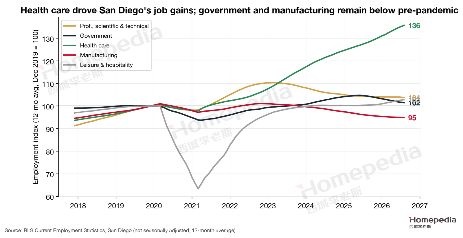
The monthly data (Figure 3) make the structure clearer. As of August 2026, health care employment was about 257,000, 34.5% above late 2019 and still up 5.0% over the year—by far the main driver of San Diego’s job growth; by QCEW, health care employment grew from 183,000 in 2019 to 222,000 in 2024, up 21.8% [1][2]. Health care growth has two long-run drivers: an aging population, since San Diego is a favored retirement destination and seniors’ medical needs keep rising; and the expansion of regional health systems and research hospitals. Like defense, health care employment is largely immune to the business cycle, giving San Diego’s housing demand a second piece of ballast. Meanwhile, professional, scientific and technical services (including biotech R&D and defense engineering services) were only 2.0% above late 2019 and down 1.8% over the year; government (including many civilian military employees) was 5.1% below late 2019; and manufacturing (including shipbuilding, aerospace and electronics) 6.6% lower [2].
These data matter for reading the map. Wei Li says “defense, biotech and R&D investment create a jobs tailwind,” and in terms of industrial base that is exactly right—these three are the sources of San Diego’s high-income jobs. But in terms of job gains since 2023, the tailwind comes mainly from health care, while defense- and research-related jobs have been flat or slightly lower. We discuss why in §3 and §4.
2.3 The Scale of High-Income Employment
Per OEWS 2025, occupations with mean pay of $150,000 or more account for about 111,000 jobs in San Diego, fewer than Dallas (about 194,000) and Boston (about 320,000) [3]. Management averages $156,776, engineering about $123,385 and healthcare practitioners about $133,746.
A relatively small pool of high-pay jobs alongside the highest prices of the three shows that San Diego’s high-end housing demand comes not only from local high-pay jobs but heavily from existing wealth: home equity built up over years of ownership, equity gains from tech and biotech companies, and outside wealth brought by retirees and remote workers. This shows up directly in the price structure in §8.
3. Defense: A Stabilizer, Not a Growth Engine
3.1 The Weight of Defense in the Regional Economy
San Diego is a principal home port of the U.S. Navy’s Pacific Fleet, with Naval Base San Diego, Naval Air Station North Island, Marine Corps Base Camp Pendleton and Marine Corps Air Station Miramar, along with General Dynamics NASSCO’s shipyard and many defense contractors. A November 2025 report by the San Diego Military Advisory Council (SDMAC) and UC San Diego’s Rady School of Management found that defense spending accounts for 22.2% of San Diego County’s gross regional product, with a total economic impact of about $61.3 billion supporting about 357,000 jobs (about 143,000 active-duty, reserve and civilian personnel, and about 214,000 indirect jobs at contractors, in logistics and in local businesses). Direct defense spending was $39.3 billion, including $19.8 billion in defense contracts, $15.1 billion in military payroll and $4.3 billion in retiree and veteran benefits; total spending was down about 3% from the prior year [4].
3.2 Contract Dollars: High but Flat, Recently Lower
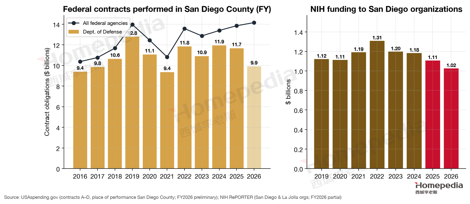
Using USAspending.gov, we tallied federal contracts with San Diego County as the place of performance (Figure 4, left) [5]. Department of Defense contracts peaked at about $12.8 billion in FY2019, were about $12.0 billion in FY2024 and about $11.7 billion in FY2025; FY2026 (just ended, with reporting incomplete) currently stands at about $9.9 billion and is expected to be revised up. Contracts from all federal agencies totaled about $13.9 billion in FY2025.
USAspending’s figure is below SDMAC’s $19.8 billion because the definitions differ: USAspending counts contracts by place of performance, while SDMAC also includes contracts awarded to local firms but partly performed elsewhere, plus other adjustments. But both point the same way: defense spending is high, but not growing, and has edged down over the past two years.
3.3 The Outlook for Defense
The direction of defense spending depends on the federal budget and strategic priorities. On one hand, U.S. strategy is shifting toward the Indo-Pacific, so demand for building, maintaining and deploying naval vessels is long-lasting, and San Diego, as the Pacific Fleet’s core home port, is well positioned. On the other hand, federal budget constraints, uncertain appropriations and reallocation among services and programs could make San Diego’s contract dollars fluctuate. SDMAC’s roughly 3% decline in total spending in 2025 and the slight decline in FY2024–2025 contracts in USAspending show that such fluctuation is already happening. Our judgment: defense’s role as a cornerstone of San Diego’s economy will not change, but for the foreseeable future it is more likely to be a stabilizer than a new driver of price gains.
3.4 Implications for Housing
Defense matters to San Diego housing mainly as a source of stability:
- A very solid floor under demand. Military personnel rotate stations on a regular schedule, so many new families arrive every year needing to rent or buy; the military’s Basic Allowance for Housing (BAH) is adjusted to local rent levels, giving the rental market steady purchasing power.
- Defense contractors provide high-pay engineering jobs. Engineers in shipbuilding, aerospace, communications and cybersecurity are important buyers of mid- to upper-priced homes.
- But it is no longer a growth engine. Flat contract dollars and government and manufacturing employment below pre-pandemic levels mean defense cannot deliver new housing demand in the near term.
We therefore read the map’s “Infrastructure upside: High” this way: defense and defense-industrial infrastructure give San Diego an unusually firm demand floor, an important reason prices are “firm”; but what it delivers is stability, not growth. If future defense budgets (especially shipbuilding and Pacific-strategy spending) expand meaningfully, this cornerstone could become a growth driver again—one trigger for the upside scenario.
4. Biotechnology and Research Funding: A Cyclical Downturn
San Diego is one of the most important life-sciences clusters in the U.S. Torrey Pines, University City (UTC) and Sorrento Valley host hundreds of biotech companies, alongside world-class research institutions such as UC San Diego, Scripps Research and the Salk Institute.
Using NIH RePORTER, we tallied NIH awards to organizations in San Diego and La Jolla (Figure 4, right) [6]: about $1.31 billion in FY2022, about $1.18 billion in FY2024, about $1.11 billion in FY2025 and about $1.03 billion in FY2026 (through early October), 13.4% below 2024; the number of funded projects fell from 2,077 in 2024 to 1,654 in 2026, down 20.4%. The decline is clearly steeper than Boston’s (Massachusetts −6.6% over the same period).
In commercial real estate, Savills reports San Diego County life-sciences vacancy of 28.1% in Q2 2026, roughly unchanged from a year earlier, with available space rising from 8.9 million to 9.4 million square feet [7]. Since the start of 2026, several local biotech companies have cut staff after clinical trial failures or funding difficulties; for example, Gossamer Bio cut about 48% of its workforce in March [8].
The link between biotech and housing is highly concentrated geographically. The research parks of Torrey Pines and UTC sit next to La Jolla, Del Mar and the North County coast, and researchers, clinical developers and managers tend to live in these communities within a 20–30-minute commute; production, lab-technician and administrative staff live more in Mira Mesa, San Marcos and inland towns. Changes in biotech financing and hiring therefore show up first in demand for mid- to upper-priced homes on the coast and in North County.
The biotech downturn’s effect on housing is concentrated along the North County coast and around UTC: researchers and biotech employees are important buyers of mid- to upper-priced homes in Carlsbad, Del Mar, La Jolla and UTC. Compared with Boston, though, San Diego’s economy depends less on life sciences, and defense and health care provide more cushion—one reason San Diego prices have plateaued at a high level since 2024 rather than falling noticeably.
5. Artificial Intelligence and the Labor Market
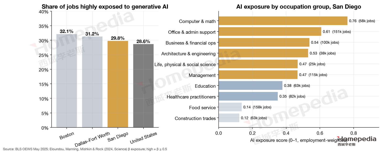
Following the method of the first two reports, we matched BLS OEWS May 2025 occupational data with the exposure scores of Eloundou et al. (2024, Science) [3][9]. In San Diego, 29.8% of jobs—about 409,000—are highly exposed, the lowest of the three metros, slightly above the U.S. (28.6%) and below Dallas (31.2%) and Boston (32.1%). This is consistent with the map’s “Med–low” rating.
San Diego’s relatively low exposure reflects more jobs that AI struggles to replace: military personnel, health care services, tourism and hospitality, construction, and many hands-on manufacturing and shipbuilding jobs. The most exposed occupational groups are computer and mathematical (0.76, about 58,000 workers), office and administrative support (0.61, about 151,000), business and financial operations (0.54, about 100,000) and engineering (0.53, about 38,000); healthcare practitioners (0.35, about 82,000), construction (0.12) and food service (0.14) are very low [3][9].
For housing, AI’s effect in San Diego will be milder than in the other two metros. Two groups deserve attention: office and administrative support workers (about 150,000), the main source of demand for entry-level homes and rentals; and engineering and R&D staff at communications-technology firms such as Qualcomm and at biotech companies—AI may raise their productivity but also reduce new hiring. Overall, AI is not a major source of risk for San Diego home prices.
6. The Marginal Buyer: Migration, Wealth and Affordability
6.1 Persistent Domestic Out-Migration
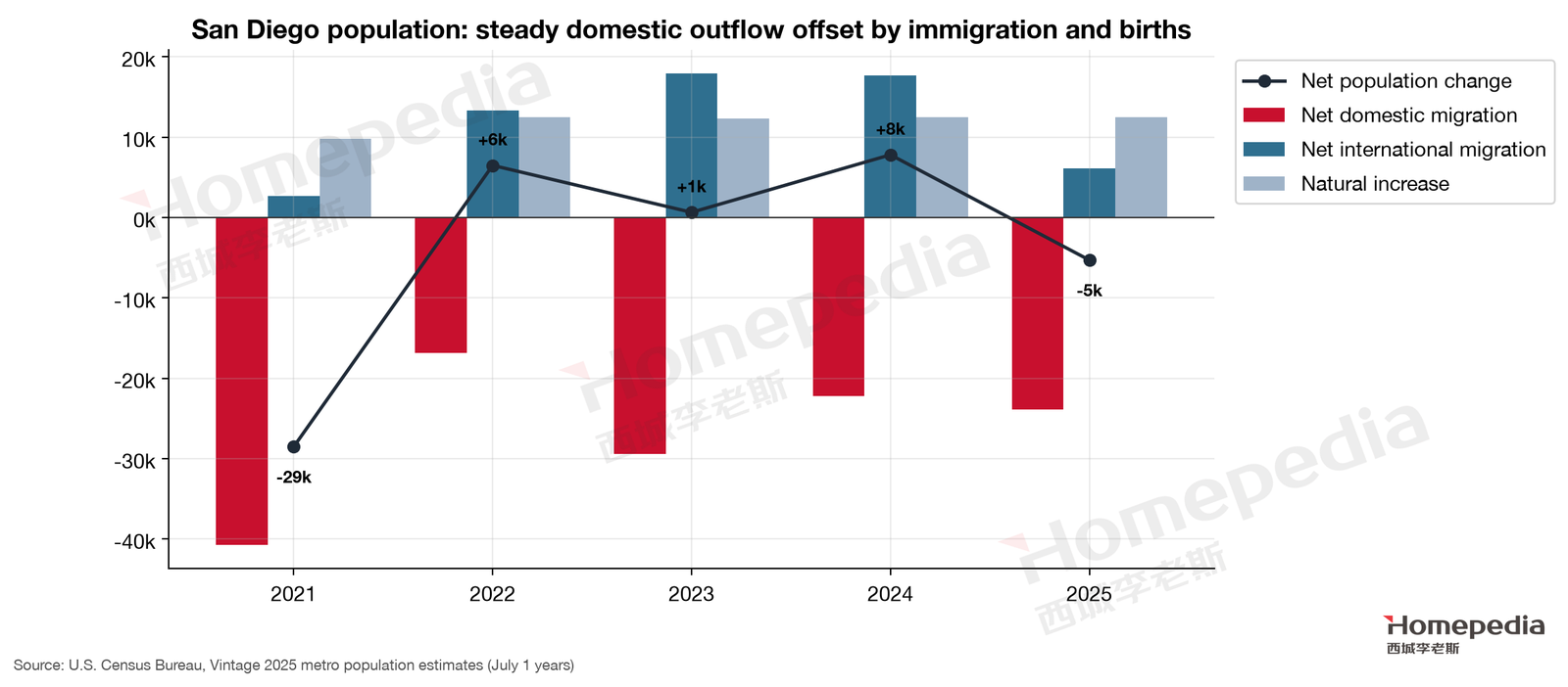
Census Vintage 2025 estimates show the San Diego metro shrinking from 3.301 million in 2020 to 3.282 million in 2025, a loss of about 19,000 over five years [10]. Net domestic migration was negative every year in 2021–2025, between −17,000 and −41,000, and −23,876 in 2025; net international migration fell from about 18,000 a year in 2023–2024 to 6,132 in 2025; natural increase was about 12,000 a year [10]. Population fell by about 5,300 in 2025. San Diego lost about 66,000 residents to net domestic migration in 2011–2019, showing this is a long-run trend.
The sharp drop in international migration in 2025 matters for the rental market: newly arrived immigrants, international students and foreign researchers almost all rent, and fewer of them slows rental demand growth in some neighborhoods—one reason San Diego’s rent growth slowed to 1–2% in 2025–2026.
A shrinking population alongside rising prices is itself a sign of supply constraints and wealth effects: those leaving are mostly low- and middle-income households who can’t afford to stay; those staying and arriving have more purchasing power.
6.2 Incomes of Arrivals and Departures
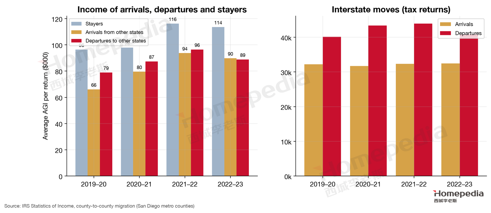
IRS county-to-county migration data show [11] that in tax year 2022–23, about 32,000 households moved into San Diego County from other states, with average adjusted gross income of $89,800; about 41,000 households moved to other states, with average income of $88,900—nearly identical; households that stayed averaged $114,000 (Figure 7). In each of the last four tax years, departures outnumbered arrivals, for a net outflow of roughly 8,000 to 12,000 tax-filing households a year.
In 2022–23, households leaving for other states went most often to Texas (5,266 households), Arizona (4,344) and Florida (3,444), followed by Washington and Nevada [11]—mostly states where housing costs clearly less than in San Diego. A substantial share of leavers are likely young and middle-income families priced out by high housing costs who rented in San Diego for years and never managed to buy. San Diego is losing precisely the people who could have become entry-level buyers, consistent with the stalling of entry-level product in §8.
These data show that the map’s “marginal affluent buyer modestly rising” does not come from interstate migration—arrivals earn about the same as departures, both well below stayers. Growth in San Diego’s high-end demand more likely comes from wealth accumulation by local high-income households (home equity, equity gains) and migration within California (for example, high-net-worth households moving from Los Angeles or the Bay Area, which the IRS “other states” category excludes). This is exactly why demand is “fragile”: wealth fluctuates with markets more than wages do.
Putting the migration data together with the price structure, San Diego’s high-end demand has roughly three sources. First, the local “property ladder”: households that bought years ago have built large home equity, and by selling and adding savings they can buy a pricier home; this trade-up demand is most active at the high end. Second, equity and tech wealth: employees of biotech, communications-technology and big tech companies hold equity, which grows quickly when stocks rise. Third, out-of-area high-net-worth households: retirees and remote workers from Los Angeles, the Bay Area and other states who bring wealth built in high-cost areas to the San Diego coast. What all three share is dependence on asset prices rather than current wages.
6.3 Housing Affordability
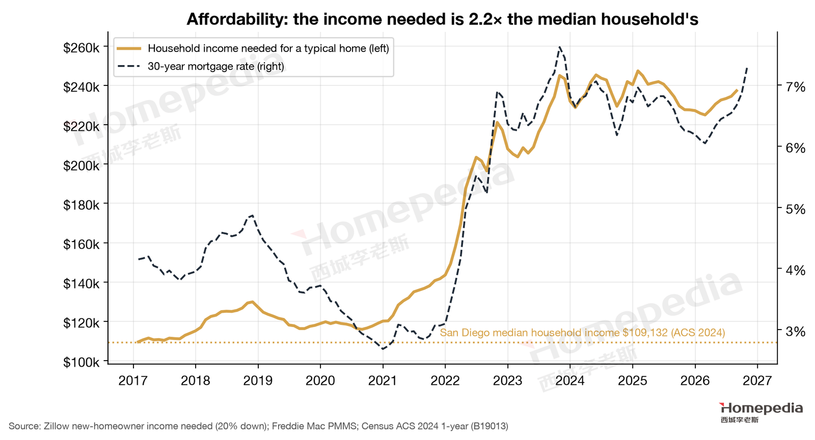
Zillow estimates that buying a typical San Diego home with 20% down, keeping payments under 30% of income, required household income of about $237,294 in August 2026, versus $118,865 in December 2019—exactly double [12]. The metro’s median household income is $109,132 (2024 American Community Survey) [13]—the income needed is 2.17 times the median, the highest of the three metros (Boston 1.66×). The typical home is 8.5 times median household income, versus 6.2× in Boston, 3.9× in Dallas and 4.5× nationally.
Box 1. Monthly Carrying Cost of a Typical Home
At San Diego’s August 2026 typical value of $930,784, with 20% down (about $186,000), a loan of about $745,000 and a 7.28% 30-year fixed rate [14]:
- Principal and interest: about $5,095 a month
- Property tax (Proposition 13 sets a base rate of 1% of the purchase price; with local bonds and assessments we estimate 1.1–1.2%; newer communities with Mello-Roos special taxes pay more): about $853–931 a month
- Homeowners insurance (assuming $1,500–3,000 a year; possibly much higher in high wildfire-risk areas): about $125–250 a month
- Total: roughly $6,070–6,280 a month (before HOA dues and maintenance)
By comparison, a typical San Diego single-family rental is about $4,136 a month and a typical home of any type about $2,993 [12]. Owning a typical home costs about $1,900–2,100 more per month in cash than renting a single-family home, plus a down payment of about $190,000—the largest own-vs-rent gap of the three metros.
Compare late 2019: the same home was worth about $603,000, the average rate was 3.72%, and principal and interest was about $2,225 a month. Prices rose 54%, but the payment rose to 2.3 times its earlier level.
6.4 Rate Lock-In and Proposition 13: The Metro Where Owners Least Want to Sell
Realtor.com data show that over the past 12 months, new listings in San Diego averaged only 65% of the same months in 2017–2019, the lowest of the three metros (Boston 79%, Dallas 96%) [15].
San Diego owners are reluctant to sell for two compounding reasons. One is nationwide rate lock-in: owners who borrowed at around 3% during the pandemic face much higher payments if they move. The other is California’s own Proposition 13: property is assessed at its purchase price, and the assessment can rise at most 2% a year thereafter. An owner who bought for $500,000 in 2010 may today be taxed on an assessed value of only about $650,000; if they sell and buy a $1 million home locally, their tax is immediately reassessed at $1 million. This double lock makes resale supply in San Diego extremely scarce and keeps sales volume depressed.
7. Housing Supply Constraints
Box 2. Why San Diego Cannot Build
San Diego’s supply constraints result from geography, institutions and risk layered on top of one another.
Geography. The city is hemmed in by the Pacific, the Mexican border, the eastern mountains and Camp Pendleton to the north; within it, dozens of canyons—mostly preserves or too steep—cannot be developed. Flat land suitable for large-scale development ran out decades ago, so new housing must infill existing neighborhoods or push east into the mountains.
Institutions. Coastal development requires approval from the California Coastal Commission; large projects must pass environmental review under the California Environmental Quality Act (CEQA), where litigation can delay projects for years; many communities have long been zoned primarily for single-family homes, and resident opposition to densification is strong.
Risk. Expanding east means entering high wildfire-risk zones. Recent updates to wildfire hazard maps have enlarged high-risk areas, insurance costs have risen, and local governments have begun limiting densification on high-risk parcels with a single access route (§7).
These three constraints make San Diego one of the hardest places in the country to build: almost every increment of demand turns into price.
7.1 Scale of New Housing Supply
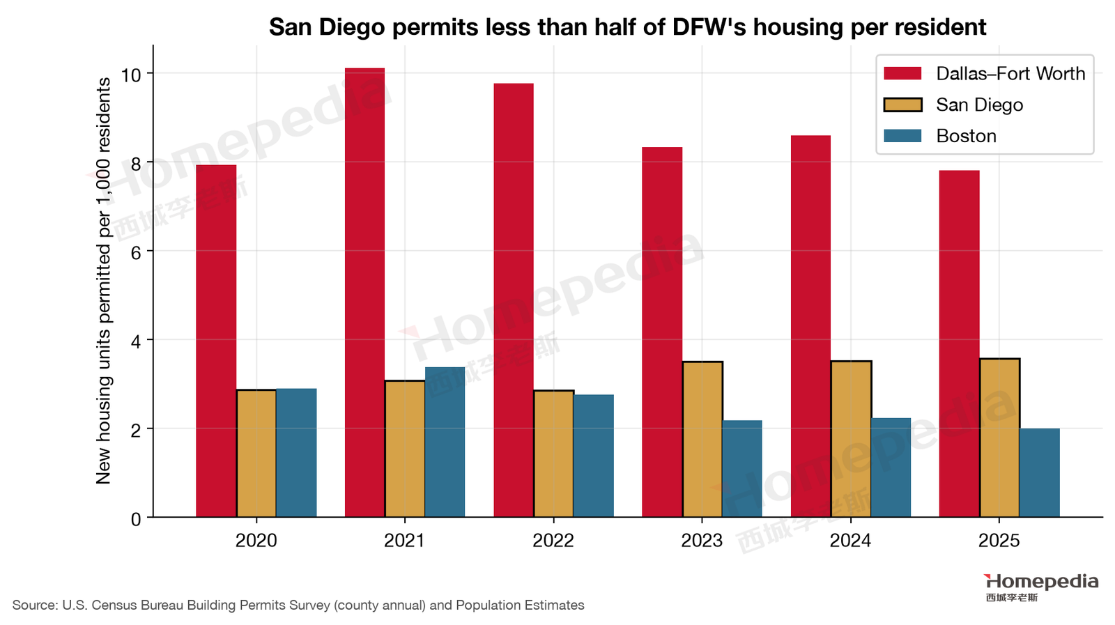
Census building permit data show San Diego County permitted 63,614 homes in 2020–2025, 69% of them multifamily [16]. Per capita (Figure 9), it permits 2.9–3.6 homes per 1,000 residents a year, less than half of Dallas (7.8–10.1) but above Boston (2.0–3.4). Notably, San Diego’s permits have risen since 2023, reaching 3.6 per 1,000 in 2025, or 11,707 homes, the highest in six years.
Part of the credit goes to a series of recent California housing reforms: easier approval of accessory dwelling units (ADUs), SB 9 allowing single-family lots to be split or to hold two homes, and the City of San Diego’s “bonus ADU” program. The reforms have met resistance, though: in 2025 the San Diego City Council voted 5–4 to amend the program, capping ADUs per lot, eliminating bonus ADUs in eight single-family zones, and excluding parcels in high wildfire-risk areas with a single access route [17]. Even at the policy level, expanding supply in San Diego is a continuing tug-of-war.
7.2 Supply Elasticity: Fifth Lowest in the Country
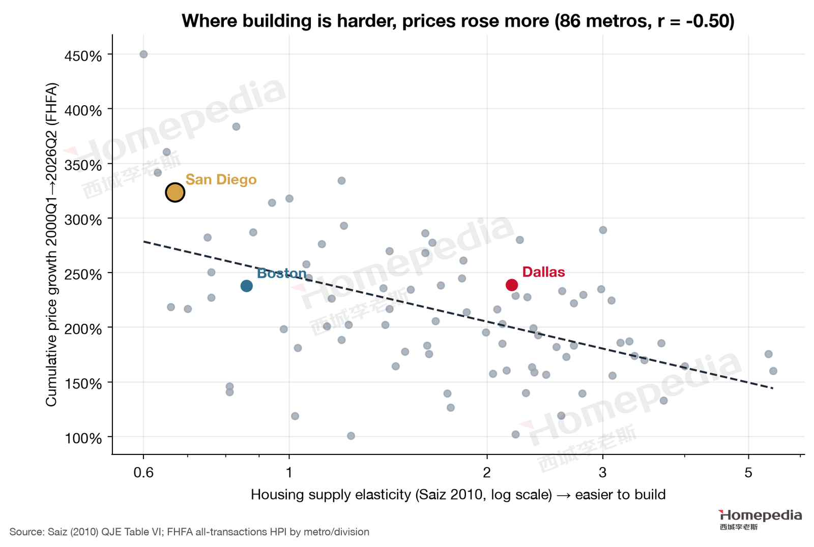
Saiz’s (2010) estimates for 95 metros put San Diego’s housing supply elasticity at 0.67, the 5th lowest in the country, behind only Miami, Los Angeles, Fort Lauderdale and San Francisco [18]. Across 86 matched metros, lower elasticity goes with larger price gains since 2000 (correlation −0.50); San Diego’s cumulative gain since 2000 of 324% sits in the upper left of the chart, far above Boston (238%) and Dallas (239%) (Figure 10) [18][19].
7.3 Limited Demand, the Largest Price Gains of the Three
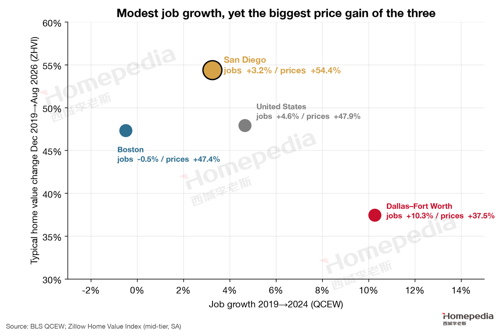
Put demand and prices together (Figure 11): San Diego’s job growth (+3.2%) trails the U.S. (+4.6%) and Dallas (+10.3%), yet its price gain (+54.4%) is the highest of the four areas compared. Through December 2024 alone, San Diego rose 57.6%, also above the U.S. (46.9%), Dallas (45.7%) and Boston (44.0%) [12].
7.4 Sensitivity of Prices to Demand: Highest of the Three
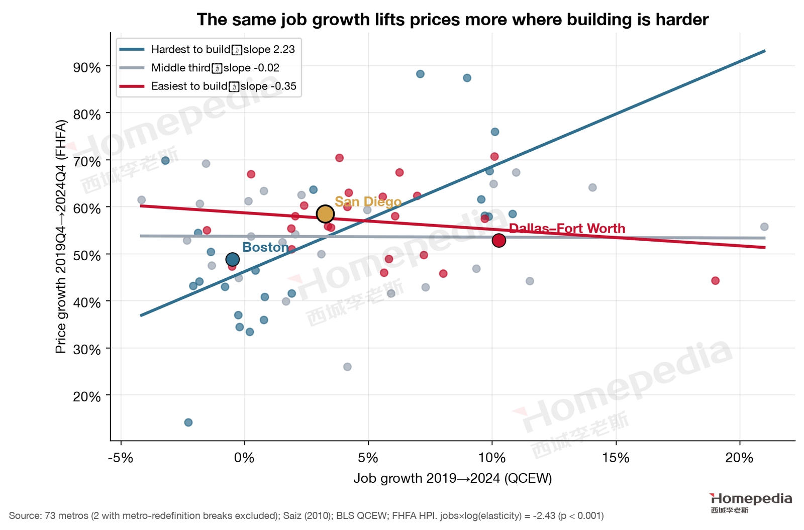
In Report No. 1’s 73-metro regression, the interaction coefficient was −2.43 (p < 0.001) [1][18][19]. Plugging in San Diego’s elasticity (0.67), the model implies that each percentage point of job growth raises San Diego prices by about 2.9 points, the highest of the three metros (Boston about 2.3, Dallas about zero) (Figure 12).
This is the mathematical meaning of “firm but fragile”: in San Diego, any growth in demand is amplified nearly threefold in prices; conversely, any contraction is amplified just the same. Because high-end demand depends mainly on wealth rather than wages, swings in equities and in tech and biotech valuations pass directly to prices through this amplifier.

8. Price Structure: The High End Leads, the Low End Stalls
8.1 Aggregate Price Trends
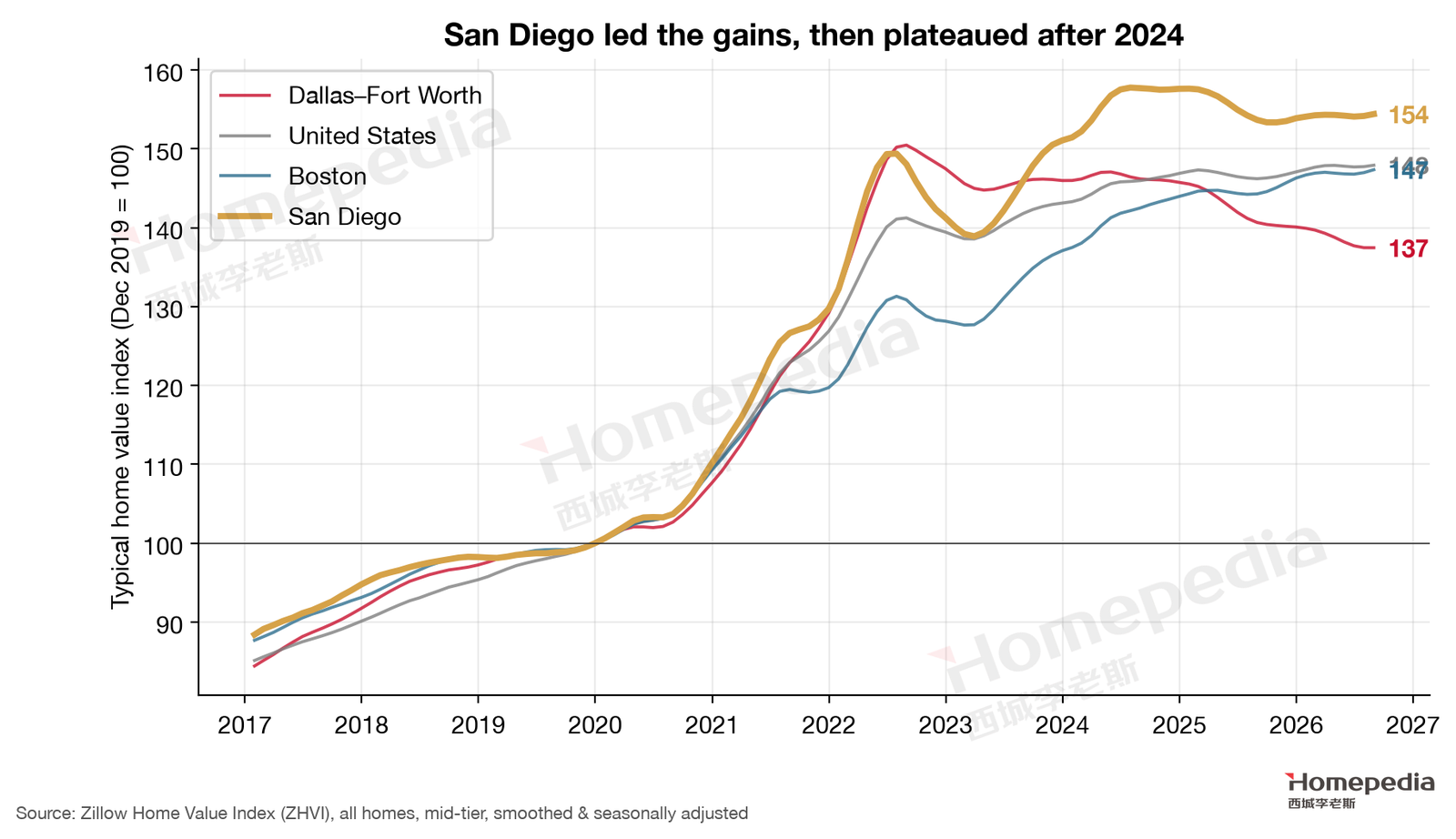
The Zillow Home Value Index shows San Diego’s typical value peaked at $951,005 in July 2024 and has plateaued since, at $930,785 in August 2026, 2.1% below peak and up 0.5% over the year [12] (Figure 14). FHFA’s repeat-sales index shows San Diego 64.3% above 2019Q4 as of 2026Q2, the highest of the three metros [19].
8.2 Inventory, Price Cuts and Pace of Sales
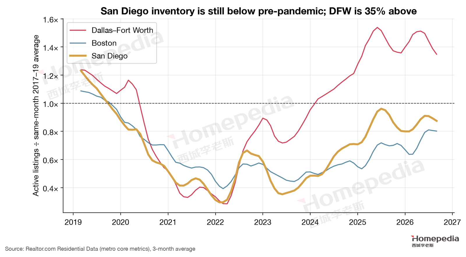
Realtor.com data show 5,749 active listings in San Diego in September 2026, about 88% of the 2017–2019 average for the same month and down 1.5% from a year earlier (Figure 15) [15]. Inventory remains below pre-pandemic, so supply scarcity has not changed.
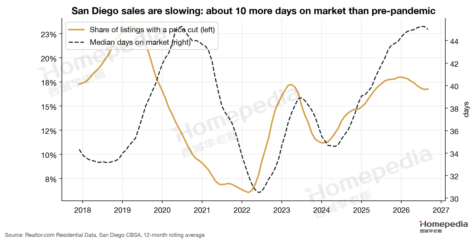
But market activity is slowing (Figure 16). In September 2026, 20.4% of San Diego listings had a price cut, above the pre-pandemic average of 18.9%; the median listing had been on the market 46 days, about 10 days longer than the pre-pandemic average of 36 [15]. This looks paradoxical: inventory is below pre-pandemic, yet homes sell more slowly. The reason is that San Diego’s “low inventory” is caused by sellers unwilling to sell (new listings are only 65% of pre-pandemic), not by buyers snapping homes up. The homes that do come to market face a shrunken pool of buyers.
Slower sales and more price cuts without rising inventory point to the buyer side: at current prices and rates, fewer buyers are willing and able to act. This is “fragility” as it shows up in transactions.
8.3 Price Tiers: Divergence Opposite to Dallas
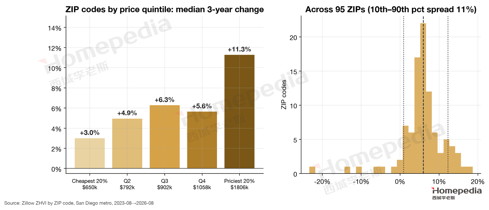
San Diego’s 95 ZIP codes with complete data show divergence exactly opposite to Dallas’s (Figure 17). From August 2023 to August 2026, the cheapest fifth (median about $650,000) rose only 3.0%, the second group 5.0%, the middle 6.3% and the fourth 5.6%, while the priciest fifth (median about $1.806 million) rose 11.3% [12]. Since late 2019, the cheapest ZIPs are up 40.9% and the priciest 75.2%.
In Dallas, new supply presses on the low end, so cheap homes fell and expensive homes held; in San Diego, there is almost no new supply, and prices are set by buyers’ ability to pay. Ordinary households’ ability to pay has hit its ceiling, so the low end stalls; high-income and high-net-worth households’ ability to pay is still growing (equities, stock compensation, home equity), so the high end leads. This “K-shaped” structure shows San Diego’s price gains increasingly depend on a small number of wealthy households.
8.4 Geographic Divergence: High-End Coastal Communities Lead
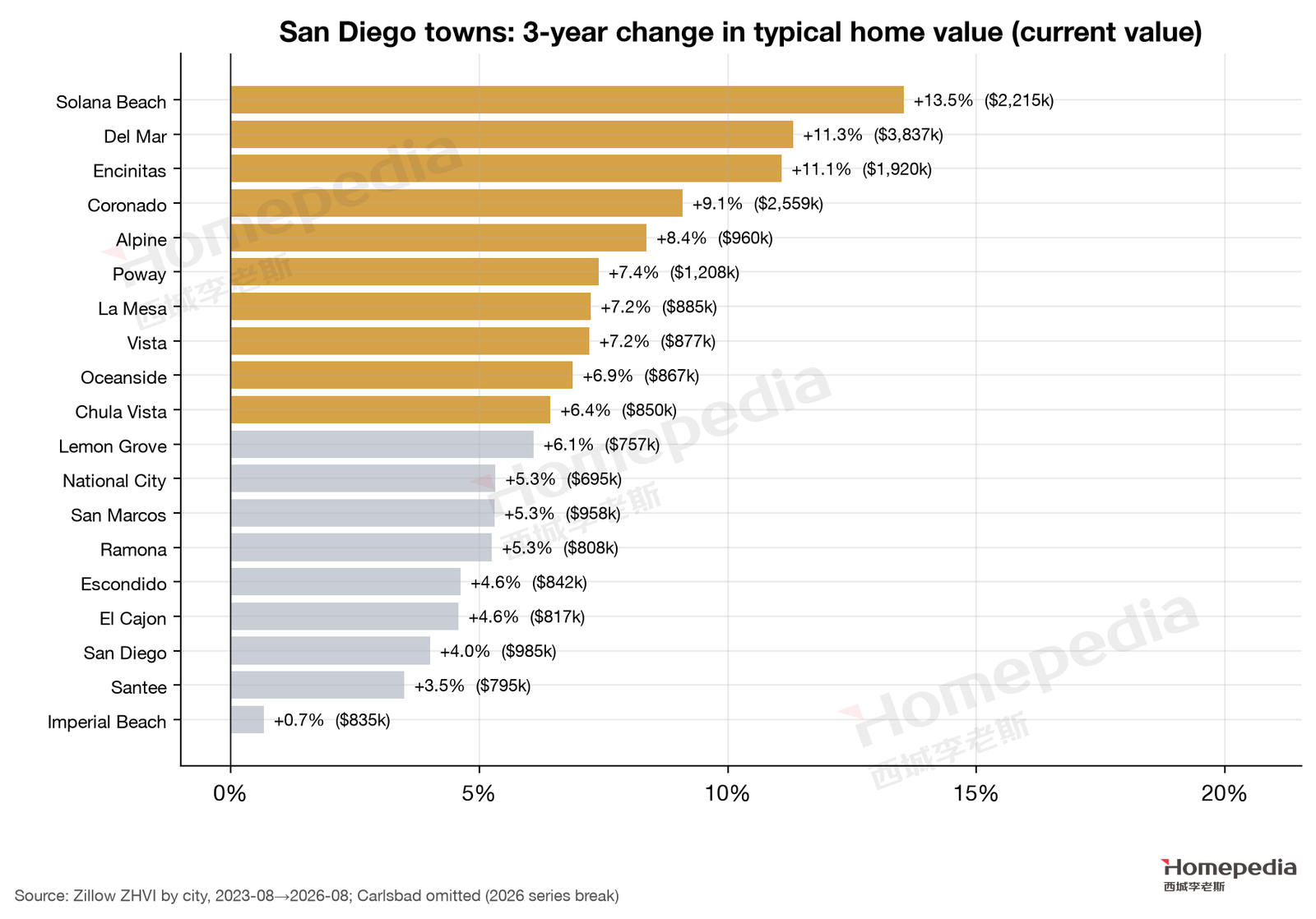
Town-level data confirm this (Figure 18). The largest three-year gains are all in high-end coastal communities: Solana Beach +13.5% (typical value about $2.21 million), Del Mar +11.3% (about $3.84 million), Encinitas +11.1% (about $1.92 million) and Coronado +9.1% (about $2.56 million). The smallest are in entry-level South Bay and East County towns: Imperial Beach +0.7%, Santee +3.5%, the City of San Diego +4.0% and El Cajon +4.6% [12]. Since 2019, Encinitas is up 75.7% and Solana Beach 74.5%, while Imperial Beach is up only 36.9%. (Carlsbad’s Zillow index shows an anomalous break in the first half of 2026 and is excluded.)
8.5 Why the High End Is Stronger: How Wealth Effects Transmit
Why, within the same metro, have the most expensive homes risen most while entry-level homes have barely moved? The key is that the two kinds of buyers face entirely different constraints.
Entry-level buyers rely mainly on wages and mortgages: how expensive a home a household can buy depends on how large a payment its income can support. When rates rose from 3% to 7%, the amount the same income could borrow fell by about 40%, and San Diego’s median household income did not rise correspondingly, so entry-level demand got “stuck.”
High-end buyers rely more on wealth: large down payments or all-cash purchases, proceeds from selling a previous home, and liquidated equity. Rising rates matter much less to them, while wealth gains from rising stocks and home values actually increase their purchasing power. That is why, after 2022, higher rates hit San Diego’s high end far less than its low end.
The risk in this structure is correlation: high-end buyers’ wealth is closely tied to equities and tech valuations. If stocks fall significantly, high-end buyers’ purchasing power shrinks together, and high-end coastal communities have almost no other kind of buyer to step in. This is why the map rates luxury single-family homes as “volatile.”
8.6 Property Type: Condos Clearly Retreating
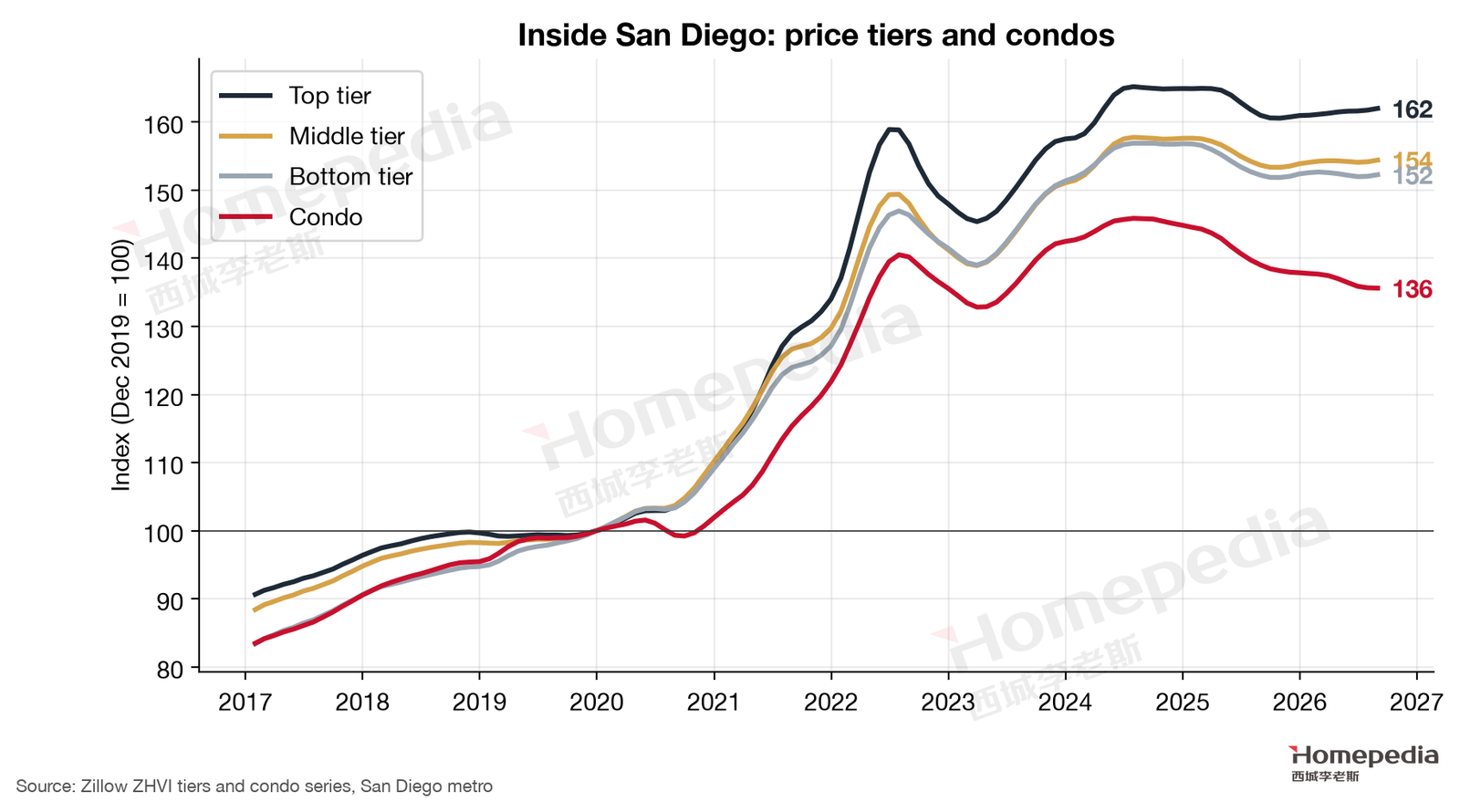
Zillow’s tiered indexes (Figure 19) show San Diego’s top tier up 62.0% since late 2019, the middle tier 54.4% and the bottom tier 52.3%, all only 2–3% below their peaks; condos are up only 35.6%, 7.0% below their July 2024 peak and down 2.5% over the year, at a typical $621,269 [12]. Condos are the main choice for San Diego’s entry-level buyers, and their retreat is the same phenomenon as the stalling of low-priced ZIPs: entry-level buyers’ ability to pay has topped out. Rising HOA dues and insurance costs (§10) further erode condo appeal.
9. The Rental Market: The Strongest Rental Demand of the Three
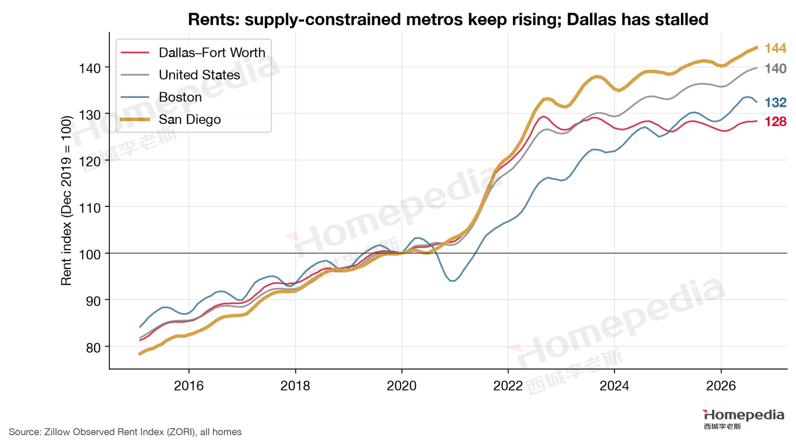
San Diego has the largest rent gains of the three metros (Figure 20): the typical rent is $2,993, 44.1% above late 2019—above the U.S. (39.7%), Boston (32.4%) and Dallas (28.3%)—and up 2.0% over the year; single-family rents are up 51.5% (about $4,136) and apartment rents 37.8% (about $2,727), still at record highs [12].
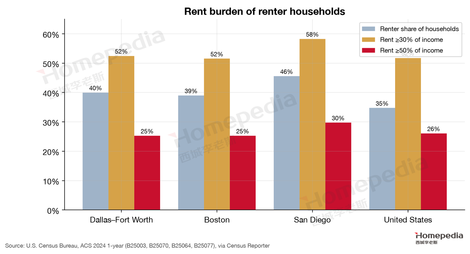
The American Community Survey shows 45.6% of San Diego metro households rent, the highest of the three (Dallas 40.0%, Boston 39.0%, U.S. 34.7%); 58.3% of renter households pay more than 30% of income in rent and 29.7% more than half, also the highest of the three (Figure 21) [13]. Median rent is $2,336 and median home value $914,700.
Town-level data show a pattern different from Boston’s. In Boston’s core, rents rose about twice as fast as home values; in San Diego, home values outpaced rents in almost every town: since late 2019, the City of San Diego’s values rose 52.1% and rents 42.1%; Chula Vista values +53.4%, rents +47.6%; Oceanside values +60.6%, rents +49.6%; Encinitas values +75.7%, rents +58.3% [12]. Both rental and owner-occupied demand are strong in San Diego, but wealth has pushed values even higher, steadily compressing rental yields—which is why San Diego rentals net only about 2.7% in the example in §13.
These data are the most direct evidence for the map’s “Rental homes: Firm”: buying requires 2.17 times median income, and nearly half of households can only rent, with no alternative even under heavy rent burdens.
In multifamily, Northmarq reports San Diego apartment vacancy of about 4.6–4.8% in Q1 2026, with net absorption of more than 3,600 units over the prior year; deliveries in 2026 will be lower than in 2025 but still well above the historical average [20]. New supply has slowed rent growth to 1–2%, but vacancy remains healthy.
Two more forces support San Diego’s rental demand. One is military housing allowances: many active-duty service members and their families rent off base, and allowances adjust to local rents, providing a steady pool of tenants who can pay in nearby communities. The other is new rental supply from ADUs: the many ADUs built in recent years are mostly rented out, adding small rental units and somewhat easing rent growth, though they remain limited relative to demand.
Student housing demand is equally strong: UC San Diego enrolled a record 45,087 students in fall 2025, with more than 2,300 still on the on-campus housing wait list; San Diego State welcomed a record 6,745 first-year students the same year and plans new residence halls for about 4,500 students [21].
10. Insurance and Wildfire Risk: A New Carrying Cost
San Diego’s distinctive risk is wildfire and insurance. In recent years many insurers have reduced or stopped renewing coverage for homes in high-risk areas of California, and more and more owners have turned to the California FAIR Plan, a state insurance pool that serves as the insurer of last resort. FAIR Plan data show that as of March 31, 2026, FAIR Plan policies in San Diego County reached 62,114, up 57.8% in a year [22].
Insurance affects prices very differently by location: insurance markets on the coast and in the city are relatively normal, while in East County mountain and high wildfire-risk areas such as Ramona, Alpine and Julian, choices have shrunk and premiums have risen sharply. For buyers this means two things: greater uncertainty about carrying costs, so buyers must confirm they can get insurance at a reasonable price before buying; and a potentially smaller buyer pool when homes in high-risk areas are resold. For condos, rising premiums on the building’s master policy pass directly into higher HOA dues.
We advise buyers to treat insurance as a transaction condition as important as financing: before making an offer, ask an insurance broker for a preliminary quote for the address; confirm the home’s wildfire hazard rating and nearby fire protection; find out whether the home has been hardened (for example, ember-resistant vents, roofing materials and defensible space around the house), which can affect premiums and insurers’ willingness to write coverage; and if only FAIR Plan basic fire coverage is available, add a difference-in-conditions (DIC) policy and count the total cost.
11. Comparative Analysis: Dallas–Fort Worth, Boston and San Diego
| Indicator | Dallas–Fort Worth | Boston | San Diego | Source |
|---|---|---|---|---|
| Job growth 2019→2024 | +10.3% | −0.5% | +3.2% | BLS QCEW [1] |
| Net domestic migration (2025) | +18,197 | −29,132 | −23,876 | Census [10] |
| Median household income (2024) | $92,733 | $117,825 | $109,132 | ACS [13] |
| Typical home value (Aug 2026) | $360,437 | $733,574 | $930,785 | Zillow [12] |
| Home value ÷ median income | 3.9× | 6.2× | 8.5× | Computed |
| Price change Dec 2019→Aug 2026 | +37.5% | +47.4% | +54.4% | Zillow [12] |
| Distance from recent peak | −8.6% | 0.0% | −2.1% | Zillow [12] |
| Permits per 1,000 residents (2025) | 7.8 | 2.0 | 3.6 | Census BPS [16] |
| Active listings ÷ pre-pandemic | ~1.35× | ~0.80× | ~0.88× | Realtor.com [15] |
| Supply elasticity (Saiz 2010) | 2.18 / 2.80 | 0.86 | 0.67 | Saiz [18] |
| Share of jobs highly exposed to AI | 31.2% | 32.1% | 29.8% | OEWS × Eloundou et al. [3][9] |
| Share of households renting | 40.0% | 39.0% | 45.6% | ACS [13] |
For investors, this table means the three metros’ risks come from entirely different places: Dallas fears oversupply, Boston fears a demand shock, and San Diego fears affordability and wealth contracting together. In San Diego, what to watch is not new supply (it will barely increase) but the wealth of high-income households and interest rates.
Of the three, San Diego is the archetypal “scarcity market”: the most constrained supply, the highest prices, the largest gains and the highest share of renters. It differs from Boston in the source of demand: Boston is supported by a large stock of high-pay jobs, San Diego more by wealth and a stable defense base. It differs from Dallas in the direction of divergence: in Dallas the low end is suppressed by new supply; in San Diego the low end is suppressed by affordability while wealth pushes the high end up.
12. Scenario Analysis and Leading Indicators
| Upside (~20%) | Base (~55%) | Downside (~25%) | |
|---|---|---|---|
| Overall price direction (12–24 months) | Gains of 4–7% | Modest gains of 0–3%, low volume | High end corrects 5–10%, overall down 2–5% |
| Conditions | Defense budget and biotech financing expand together; rates below 6%; strong stocks | Stable defense and health care jobs; rates 6.5–7.5%; steady stocks | Biotech financing and stocks weaken; defense contracts keep falling; rates above 7.5% |
| High-end coastal single-family | Leads gains | Firm but volatile | Corrects first |
| Primary homes | Modest gains | Flat | Mild correction |
| Condos | Stop falling | Remain weak | Fall another 5–10% |
| Rental homes | Rent growth accelerates | Modest rent growth | Flat rents |
Base case: slow and firm (~55%). Supply can barely increase, owners won’t sell because of rate lock-in and Proposition 13, and inventory is below pre-pandemic, so overall prices are hard to push down meaningfully. But buying requires 2.17 times median income and rates are above 7%, so buyers are limited, volume and liquidity stay low, and days on market may stay elevated. Stable employment from defense and health care, plus wealth accumulation by local high-income households, is enough to support modest overall gains; high-end coastal communities are strongest, entry-level product and condos weak.
In this scenario, the market’s most visible feature is poor liquidity: good homes remain scarce, but buyers and sellers are both waiting, and transactions take longer. For buyers, this means room to negotiate better terms, but no reason to expect large price drops; for sellers, it means pricing more realistically and allowing more time to sell. For renters, rents will keep rising modestly at 1–3% a year, and the large own-vs-rent gap will not close soon.
Upside: firm (~20%). The trigger is three tailwinds at once: a meaningful expansion of the defense budget (especially shipbuilding and Pacific-strategy spending), a biotech financing recovery that drives hiring, and rates falling below 6%. With San Diego’s price amplifier, prices could rise 4–7%, and entry-level product would follow.
Downside: high end corrects first (~25%). The trigger is pressure on both wealth and income of high-income households: a significant stock-market correction, wider biotech layoffs, continued declines in defense contracts, and rates staying above 7.5%. Because San Diego’s high-end demand depends heavily on wealth, high-end coastal communities would adjust first and most; condos and entry-level product, already weak, would remain under pressure. But because supply is extremely scarce, owners are generally low-leverage and Proposition 13 provides a tax advantage, we do not expect widespread forced selling.
The most important signal of which scenario San Diego is moving toward is whether the gap between the high end and the low end keeps widening or starts to narrow. If rates fall and entry-level buyers return, low-priced segments and condos will stop falling and recover first, narrowing the gap from below—a signal of the upside scenario. If stocks and tech valuations weaken, days on market and price cuts in high-end coastal communities will rise first, narrowing the gap from above—a signal of the downside scenario.
Eight leading indicators readers can track each quarter (upside / downside thresholds in parentheses):
- DoD contracts performed in San Diego County (USAspending, by fiscal year): back above $12 billion upside; below $10 billion downside. FY2025: about $11.7 billion.
- NIH funding to San Diego organizations (NIH RePORTER): back above $1.2 billion upside; below $1.0 billion downside. FY2026: about $1.03 billion.
- Life-sciences vacancy (brokerage quarterly reports): below 20% upside; above 30% downside. Q2 2026: 28.1%.
- San Diego nonfarm job growth, year over year (BLS CES): >1.5% upside; <0% downside. August 2026: about +1%.
- 30-year fixed mortgage rate (Freddie Mac): <6% upside; >7.5% downside. October 1, 2026: 7.28%.
- Median days on market (Realtor.com): back below 40 days upside; above 55 days downside. September 2026: 46 days.
- Condo price index, year over year (Zillow): turning positive upside; declines widening beyond −5% downside. August 2026: −2.5%.
- FAIR Plan policies (cfpnet.com, quarterly): slower growth signals the insurance market stabilizing; continued rapid growth signals rising carrying-cost risk. March 2026: 62,114, up 57.8% year over year.
13. Outlook by Property Type
| Property type | Map view | Report conclusion | Key evidence |
|---|---|---|---|
| Luxury single-family | Volatile | Strongest but most fragile | Priciest fifth of ZIPs +75.2% since 2019; coastal communities +9–13.5% over three years |
| Primary homes | Stable | Stable, limited upside | Cheapest fifth of ZIPs +3.0% over three years; South Bay and East County towns rose least |
| Condos | Neutral | Neutral to weak | 7.0% below peak, −2.5% over the year; rising HOA and insurance costs |
| Rental homes | Firm | Firm, strongest of the three | 45.6% of households rent; 58% rent-burdened; rents +44% since 2019 |
| Student housing | Selectively firm | Firm, depends on the school | Record UCSD enrollment of 45,087; 2,300 on the campus housing wait list |
| Multifamily | Firm | Firm, but heavy near-term deliveries | Vacancy about 4.6–4.8%; 2026 deliveries still above historical average |
Luxury single-family. The map calls this segment “volatile: scarce but highly dependent on marginal affluent buyers.” The data fully support this: high-end coastal communities are San Diego’s best-performing product, but their demand comes from wealth rather than wages, so changes in stocks and tech valuations pass straight through. For long-term holders, the absolute scarcity of coastal land is the best store of value; for short-term investors, this segment is the most volatile.
Primary homes ($700,000–$1,000,000). This is where most San Diego households compete, and where affordability bites hardest. Buyers here are mainly dual-income households and mid-level employees of the military and health systems, who are most sensitive to rates: each percentage point drop in rates raises their purchasing power by about 10%, so this segment will be the first to revive when rates fall. Prices in the South Bay (Chula Vista, National City), East County (El Cajon, La Mesa, Santee) and inland North County (Escondido, San Marcos) rose only 3–7% over three years. Scarce supply holds up the floor, but payments cap the upside.
Condos. The map’s view is “neutral: steady entry-level demand, but be careful with HOA costs.” Condos are already 7% below peak, somewhat weaker than that view, so we adjust it to “neutral to weak.” Condo buyers should look closely at HOA finances and the building’s insurance renewals: rising master-policy premiums pass through to higher HOA dues and can even trigger special assessments.
Rental homes. San Diego has the strongest rental demand of the three metros, but returns are equally squeezed by high prices:
Example: the return on a typical single-family rental
Purchase price $930,784, rent $4,136 a month, annual rent $49,632: a gross yield of about 5.3%. Subtract property tax (at 1.2%) of about $11,170, insurance of about $3,000, and vacancy, repairs and management (20% of rent) of about $9,930, and net operating income is about $25,540—a net yield of about 2.7%, the lowest of the three metros (Dallas about 3.3%, Boston about 3.1%) and far below the 7.28% mortgage rate. Rental investing in San Diego depends almost entirely on long-run appreciation and rent growth rather than cash flow; Proposition 13 keeps long-term holders’ property taxes low, a structure that rewards holding longer.
Student housing. Enrollment at both UC San Diego and San Diego State is at record highs, on-campus housing has long fallen short, and student rental demand around campus (La Jolla, UTC, the College Area) is very stable.
Multifamily. Demand is the best of the three metros, but 2025–2026 deliveries remain above the historical average, so rent growth will stay low in the near term. In the long run, the supply-constrained structure won’t change, and multifamily in good locations remains firm. Areas with concentrated new deliveries face more vacancy pressure, while coastal communities and established suburbs, with few new projects and steady demand, usually have lower vacancy. In multifamily investing, location differences matter more than the metro average.
14. Strategic Implications for Market Participants
14.1 Buyers
- Confirm insurance first, then negotiate price. Especially for homes in East County, the mountains and along canyon edges, get an acceptable insurance quote before signing.
- Use the slowdown to negotiate terms. Homes sit 10 days longer than before the pandemic and price cuts are rising, so buyers have more room than in 2021–2023; homes listed more than 45 days are candidates for more assertive offers.
- Understand the long-term significance of Proposition 13. The purchase price sets the tax base for decades; for long-term owner-occupants, part of a higher purchase price is offset by years of lower taxes. In new communities, check for Mello-Roos and other special taxes.
- Entry-level buyers can consider condos, with thorough due diligence. Condos are 7% off their peak, a rare negotiating window in recent years—provided the HOA is financially healthy, insurance is stable and no major repairs are planned.
- Consider homes with an ADU or room to add one. California’s ADU approvals are relatively permissive, and a rentable accessory unit can help cover the mortgage; first confirm the lot is not in a high wildfire-risk zone or restricted by the City of San Diego’s 2025 rules.
- Look for value in the South Bay and inland North County. Chula Vista, San Marcos and Escondido cost less than half as much as coastal communities and have job and transportation support.
14.2 Sellers
- High-end sellers should act while the market is strong. High-end coastal prices are near records, but this segment’s demand depends most on stocks and wealth; if you already plan to sell, there is no need to wait for higher prices.
- Entry-level and condo sellers need accurate pricing. Buyers’ ability to pay has topped out in this segment, and overpricing leads to long listing times.
- Prepare for a longer sale. Days on market are about 10 days above pre-pandemic; allow more time, and complete necessary repairs and fire hardening before listing to improve buyers’ access to insurance.
- Consider the Proposition 13 tax-base effect. If you sell and buy again in California, your property tax resets to the new price; owners 55 and older should look into Proposition 19’s rules on transferring their tax base.
14.3 Investors
- San Diego is an asset-allocation market, not a cash-flow market. Rentals net about 2.7%, suitable only for all-cash or low-leverage investors targeting long-run appreciation.
- Rental demand is steadiest near universities and military installations. Demand around UCSD and the naval bases is less sensitive to the business cycle, and military housing allowances provide steady purchasing power.
- Coastal land is the asset with the highest long-run allocation value. Coastal land can almost never be added to, making it the scarcest asset of the three metros over the long run; it suits investors with a long horizon who can tolerate short-term swings, not strategies that rely on short-term gains or cash flow.
- Watch changes in California housing law. California passes new laws affecting ADUs, zoning and tenant protections every year; before investing in rentals, understand local limits on rent increases and eviction protections, which directly affect returns.
- Avoid areas with high insurance risk. The cost and availability of insurance in high wildfire-risk areas is the biggest uncertainty for long-term holding.
- A note for Chinese investors. California’s transaction process, disclosure requirements (such as natural hazard disclosures) and Coastal Commission planning limits are complex, and laws and tax rules affecting foreign buyers are changing; before transacting, retain a local agent and attorney to confirm current requirements.
15. Limitations and Risks
- The wealth dependence of high-end demand is hard to measure directly. We infer from price structure and migration data that high-end demand comes from wealth, but lack direct data on household wealth.
- Policy uncertainty in the defense budget. Defense spending depends on the federal budget and geostrategy and could move beyond this report’s scenarios, in either direction.
- The insurance market is still evolving. California is pursuing insurance regulatory reform; rapid growth in FAIR Plan policies may slow or continue, which would significantly affect prices in high-risk areas.
- California housing policy could speed up supply. California keeps passing laws to loosen zoning and speed approvals; if these reforms take hold much faster in San Diego, supply elasticity could exceed historical estimates and the upward pressure on prices would weaken.
- Data limitations. Carlsbad’s Zillow town series has a break and is excluded; each ZIP-code group has only 19 ZIP codes, a small sample; FY2026 NIH and USAspending data are incomplete; QCEW and CES use different definitions.
Even so, we believe the report’s core logic—topographically determined extreme scarcity keeps San Diego prices firm over the long run, while extremely low affordability and dependence on affluent wealth make the market unusually fragile—rests on basic facts of geography and market structure and will hold for the foreseeable future.
Appendix A: Methodology and Data Sources
Employment and wages. Metro employment comes from BLS QCEW annual averages for 2019 and 2024; monthly trends from BLS CES, with total employment seasonally adjusted and industry series as 12-month moving averages of non-seasonally-adjusted data.
Defense and research. Defense economic impact comes from the 2025 SDMAC and UC San Diego Rady School of Management report; federal contracts from USAspending.gov (contract award types A–D, place of performance San Diego County, summed by fiscal year; FY2026 preliminary); NIH awards from the NIH RePORTER API (organizations in San Diego or La Jolla); life-sciences vacancy from Savills’ Q2 2026 report.
AI exposure. BLS OEWS May 2025 occupational data matched to the β exposure scores of Eloundou et al. (2024), covering 90.8% of San Diego employment; “highly exposed” means β ≥ 0.5.
Population and migration. Population and components come from Census Vintage 2025 metro estimates; migration income from IRS county-to-county migration data, where “other states” means U.S. states other than California (and therefore excludes migration within California).
Housing supply. Building permits come from Census BPS (San Diego County); supply elasticity from Saiz (2010); the cross-metro regression method is described in Report No. 1’s appendix.
Prices, rents and inventory. Zillow ZHVI (metro, ZIP and town; the ZIP analysis covers 95 ZIP codes; Carlsbad excluded from the town chart because of a series break) and Zillow ZORI; Realtor.com metro core metrics (the new-listings comparison uses the ratio of the past 12 months to the 2017–2019 average for the same months); affordability from Zillow’s new-homeowner income needed; income, renter share and rent burden from ACS 2024 one-year estimates.
Reproducibility. All download scripts, charting code, raw data and intermediate statistics are archived in the project’s scripts/ (city_figures.py, fetch_bos_sd.py) and shared_data/ directories.
Data cutoffs. QCEW 2024; CES August 2026; OEWS May 2025; population estimates July 2025; IRS migration 2022–23; FHFA 2026Q2; Zillow August 2026; Realtor.com September 2026; NIH and USAspending early October 2026; mortgage rate October 1, 2026.
References
[1] U.S. Bureau of Labor Statistics. Quarterly Census of Employment and Wages, annual averages 2019 and 2024. https://www.bls.gov/cew/ [2] U.S. Bureau of Labor Statistics. Current Employment Statistics (State and Metro Area), San Diego-Chula Vista-Carlsbad, CA, through August 2026. https://www.bls.gov/sae/ [3] U.S. Bureau of Labor Statistics. Occupational Employment and Wage Statistics, May 2025. https://www.bls.gov/oes/ [4] San Diego Military Advisory Council & UC San Diego Rady School of Management. (2025, November). 2025 San Diego Military Economic Impact Report. https://sdmac.org/wp-content/uploads/2025/11/2025-SDMAC-Report-WEB-Single.pdf ; Times of San Diego (2025, November 12). Report: Military spending makes up 22.2% of regional economy. [5] USAspending.gov. Spending by geography and awarding agency, contract award types A–D, place of performance San Diego County, CA, fiscal years 2016–2026. https://www.usaspending.gov/ [6] National Institutes of Health. NIH RePORTER (API v2), projects with organization city San Diego or La Jolla, CA, fiscal years 2019–2026. https://reporter.nih.gov/ [7] Savills. (2026). San Diego life sciences market report, Q2 2026. https://www.savills.us/ [8] BioSpace. Layoff tracker (Gossamer Bio, March 2026). https://www.biospace.com/biospace-layoff-tracker [9] Eloundou, T., Manning, S., Mishkin, P., & Rock, D. (2024). GPTs are GPTs: Labor market impact potential of LLMs. Science, 384(6702), 1306–1308. [10] U.S. Census Bureau. Metropolitan Population Totals and Components of Change, Vintage 2025 and Vintage 2020. https://www.census.gov/programs-surveys/popest.html [11] Internal Revenue Service, Statistics of Income. County-to-County Migration Data, 2019–2020 through 2022–2023 (inflow and outflow files). https://www.irs.gov/statistics/soi-tax-stats-migration-data [12] Zillow Research. ZHVI (metro, ZIP, city), ZORI (metro, city), and affordability series, through August 2026. https://www.zillow.com/research/data/ [13] U.S. Census Bureau. American Community Survey 2024 1-Year Estimates, Tables B19013, B25003, B25064, B25070, B25077 (via Census Reporter). https://censusreporter.org [14] Freddie Mac. Primary Mortgage Market Survey, week of October 1, 2026. https://www.freddiemac.com/pmms [15] Realtor.com Economic Research. Residential Data, Metro Core Metrics, through September 2026. https://www.realtor.com/research/data/ [16] U.S. Census Bureau. Building Permits Survey, county annual files 2015–2025. https://www.census.gov/construction/bps/ [17] City of San Diego Planning Department. (2025). ADU regulations amendment (Report to the Planning Commission No. PC-25-016; Ordinance O-2025-136). https://www.sandiego.gov/sites/default/files/2025-04/planning-commission-report-no-pc-25-016_0.pdf [18] Saiz, A. (2010). The geographic determinants of housing supply. Quarterly Journal of Economics, 125(3), 1253–1296. [19] Federal Housing Finance Agency. House Price Index, All-Transactions, metropolitan statistical areas, through 2026Q2. https://www.fhfa.gov/data/hpi [20] Northmarq. (2026, May 5). San Diego multifamily inventory growth remains elevated, Q1 2026. https://www.northmarq.com/insights/insights/san-diego-multifamily-inventory-growth-remains-elevated-q1-2026 [21] UCSD Guardian (2026, January 12). UC fall 2025 enrollment numbers reach record high; CBS 8. Thousands of UC San Diego students on campus housing wait list; Axios San Diego (2025). San Diego State University draws record applications; CRE Daily. San Diego State University plans $1B in student housing. [22] California FAIR Plan Association. Key statistics & data: policies in force by county (as of March 31, 2026). https://www.cfpnet.com/key-statistics-data/
Disclaimer: This report is for research and educational purposes only and does not constitute investment, legal or tax advice. Real estate investing involves risk; readers should consider their own circumstances and consult licensed professionals.
Leave your email to download the 39-page report
The PDF keeps the full layout for saving and offline reading.
© 2026 Wei Li · Homepedia. All rights reserved. The text, data and charts in this report are protected by copyright and may not be copied, republished, excerpted or used commercially without written permission.
Want to know what this means for your own buying, selling or investing decision? Book a consultation